Probability

Next, we will discuss the terminology related to probability theory. Probability theory is a vital part of machine learning, as modeling data with probabilistic models allows us to draw conclusions about how uncertain a model is about some predictions. Consider the example, where we performed sentiment analysis in Chapter 11, Current Trends and the Future of Natural Language Processing where we had an output value (positive/negative) for a given movie review. Though the model output some value between 0 and 1 (0 for negative and 1 for positive) for any sample we input, the model didn't know how uncertain it was about its answer.

Let's understand how uncertainty helps us to make better predictions. For example, a deterministic model might incorrectly say the positivity of the review, I never lost interest, is 0.25 (that is, more likely to be a negative comment). However, a probabilistic model will give a mean value and a standard deviation for the prediction. For example, it will say, this prediction has a mean of 0.25 and a standard deviation of 0.5. With the second model, we know that the prediction is likely to be wrong due to the high standard deviation. However, in the deterministic model, we don't have this luxury. This property is especially valuable for critical machine systems (for example, terrorism risk assessing model).

To develop such probabilistic machine learning models (for example, Bayesian logistic regression, Bayesian neural networks, or Gaussian processes) you should be familiar with the basic probability theory. Therefore, we provide some basic probability information here.

Random variables

A random variable is a variable that can take some value at random. Also, random variables are represented as x₁, x₂, and so on. Random variables can be of two types: discrete and continuous.

Discrete random variables

A discrete random variable is a variable that can take discrete random values. For example, trials of flipping a coin can be modeled as a random variable, that is, the side of the coin it lands on when you flip a coin is a discrete variable as the values can only be heads or tails. Alternatively, the value you get when you roll a die is discrete, as well, as the values can only come from the set, {1,2,3,4,5,6}.

Continuous random variables

A continuous random variable is a variable that can take any real value, that is, if x is a continuous random variable:

Here, R is the real number space.

For example, the height of a person is a continuous random variable as it can take any real value.

The probability mass/density function

The probability mass function (PMF) or the probability density function (PDF) is a way of showing the probability distribution over different values a random variable can take. For discrete variables, a PMF is defined and for continuous variables, a PDF is defined. Figure A.1 shows an example PMF:

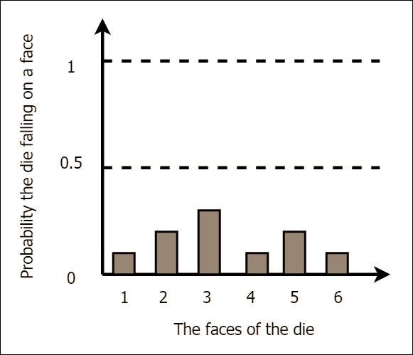
A.1: Probability mass function (PMF) discrete

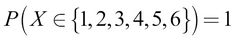
The preceding PMF might be achieved by a biased die. In this graph, we can see that there is a high probability of getting a 3 with this die. Such a graph can be obtained by running a number of trials (say, 100) and then counting the number of times each face fell on top. Finally, divide each count by the number of trials to obtain the normalized probabilities. Note that all the probabilities should add up to 1, as shown here:

The same concept is extended to a continuous random variable to obtain a PDF. Say that we are trying to model the probability of a certain height given a population. Unlike the discrete case, we do not have individual values to calculate the probability for, but rather a continuous spectrum of values (in the example, it extends from 0 to 2.4 m). If we are to draw a graph for this example like the one in Figure A.1, we need to think of it in terms of infinitesimally small bins. For example, we find out the probability density of a person's height being between 0.0 m-0.01 m, 0.01-0.02 m, ..., 1.8 m-1.81 m, …, and so on. The probability density can be calculated using the following formula:

Then, we will plot those bars close to each other to obtain a continuous curve, as shown in Figure A.2. Note that the probability density for a given bin can be greater than 1 (since it's density), but the area under the curve must be 1:

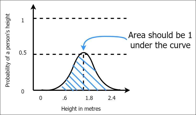
Figure A.2: Probability density function (PDF) continuous

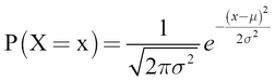
The shape shown in Figure A.2 is known as the normal (or Gaussian) distribution. It is also called the bell curve. We previously gave just an intuitive explanation of how to think about a continuous probability density function. More formally, a continuous PDF of the normal distribution has an equation and is defined as follows. Let's assume that a continuous random variable X has a normal distribution with mean and standard deviation . The probability of X = x for any value of x is given by this formula:

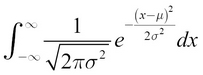
You should get the area (which needs to be 1 for a valid PDF) if you integrate this quantity over all possible infinitesimally small dx values, as denoted by this formula:

The integral of the normal for the arbitrary a, b values is given by the following formula:

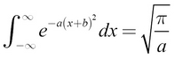
(You can find more information at http://mathworld.wolfram.com/GaussianIntegral.html, or for a less complex discussion, refer to https://en.wikipedia.org/wiki/Gaussian_integral.)

Using this, we can get the integral of the normal distribution, where and :

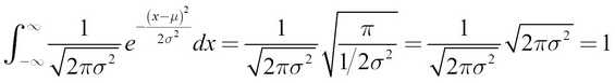
This gives the accumulation of all the probability values for all the values of x and gives you a value of 1.

Conditional probability

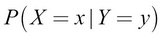
Conditional probability represents the probability of an event happening, given the occurrence of another event. For example, given two random variables, X and Y, the conditional probability of X = x, given that Y = y, is denoted by this formula:

A real-world example of such a probability would be as follows:

Joint probability

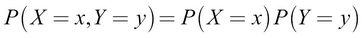
Given two random variables, X and Y, we will refer to the probability of X = x together with Y = y as the joint probability of X = x and Y = y. This is denoted by the following formula:

If X and Y are mutually exclusive events, this expression reduces to this:

A real-world example of this is as follows:

Marginal probability

Marginal probability distribution is the probability distribution of a subset of random variables, given the joint probability distribution of all variables. For example, consider that two random variables, X and Y exist, and we already know and we want to calculate P(x):

Intuitively, we will take the sum over all possible values of Y, effectively making the probability of Y = 1. This gives us

.

Bayes' rule

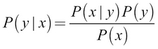
Bayes, rule gives us a way to calculate if we already know , and . We can easily arrive at Bayes' rule as follows:

Now let's take the middle and right parts:

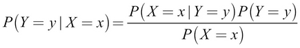
This is Bayes' rule. Let's put it simply, as shown here: