Familiarizing yourself with RStudio

Compared to RStudio, the Python development process that has been used in previous chapters has been a bit indirect. Code has been written in a text editor to perform a particular function and then executed as a whole through a separate interface.

Writing code in RStudio is more of an iterative process. Code can be run line by line from the editor, and data and variables are stored continuously within the environment. This means that you can conduct analysis, observe the data, and verify the correctness of your code as you go. The following steps can be used to create an R script in RStudio.

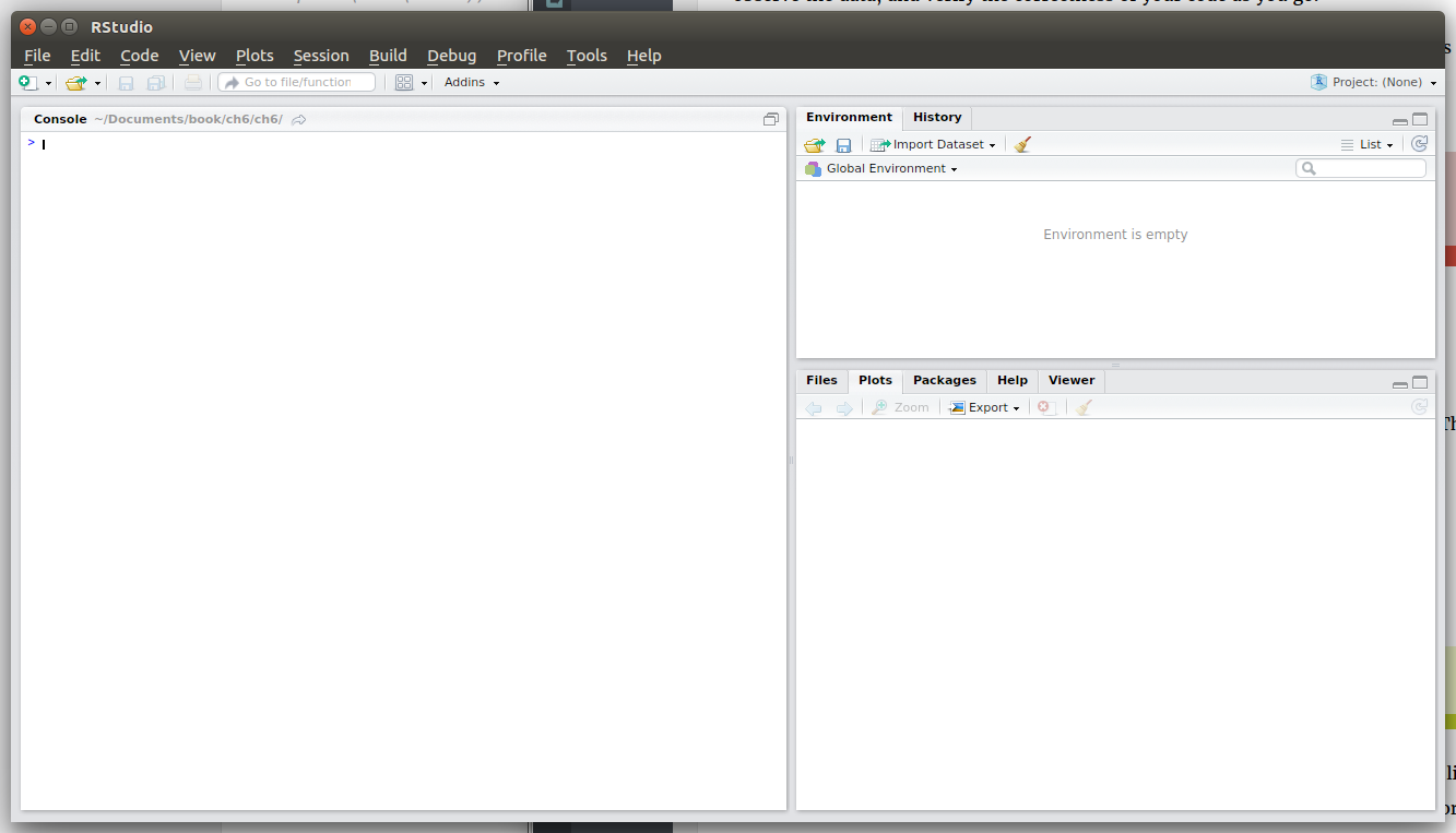
1. To begin with, open the RStudio program:

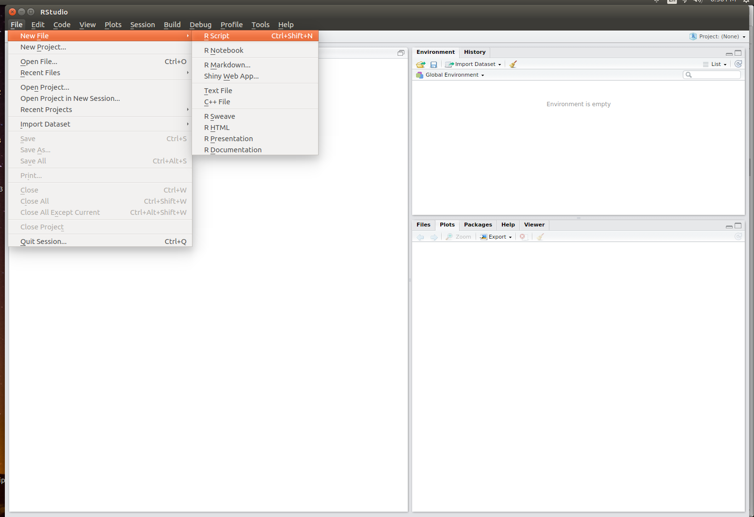
2. From RStudio, you can create a new R script by selecting File | New | Rscript. This will create and open a .R file in the text editor:

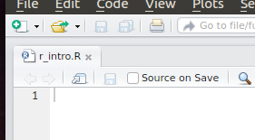
3. This will open the script for editing. You can save the script to your ch6 folder by selecting File | Save. The name of the script is not that important here, but I will name mine r_intro. Note that RStudio will add the file extension automatically:

Running R commands

Commands in R can be entered directly into the console, but they can also be run line by line from the editor. To run a line of code from the editor, you can move the cursor to that line, and press Ctrl + Enter on your keyboard.

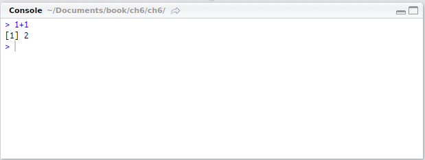
Try entering 1+1 in your R script and pressing Ctrl + Enter, with the cursor on that line. The following should be printed in the console:

Setting the working directory

Like the terminal, the R environment interacts with the filesystem relative to a particular directory. In R, the directory can be set directly in the script using the setwd() function. 

It is helpful to set the working directory at the beginning of an R script to the location of the data. For this chapter, the working directory should be set to the ch6 project folder. I've added the following line to the beginning of my script - note that the path you use should be specific to the way your file system is set up:

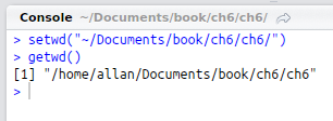
setwd("~/Documents/book/ch6/ch6/")

In R, the forward slash / character can be used regardless of operating system. After adding a line to set the working directory, you can execute the line by moving the cursor to that line and pressing Ctrl + Enter. Alternatively, you can highlight some or all of the text from one or more lines and press Ctrl + Enter to execute the code. If the command works, you should see the line printed in the console below the editor. You can verify that the working directory is set correctly by entering getwd() into the console as follows:

Reading data

You can read a CSV dataset into the R environment using the read.csv() function, which accepts a path string to a CSV file and returns an R dataframe. Variable assignment in R is done using the <- symbol, which is more or less analogous to the = symbol in Python. After the working directory is properly set, the following line will read artificial_roads_by_region.csv and assign the resulting data to an R dataframe called roads:

roads <- read.csv("data/artificial_roads_by_region.csv")

The R dataframe

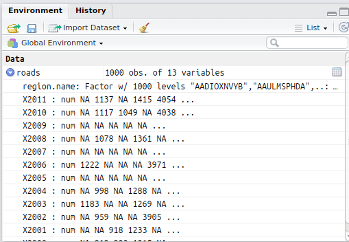
The R dataframe is a built-in data structure that represents tabular data. Once a dataframe is created, the columns and initial values of the dataframe can be viewed in the Environment tab in the upper left corner of RStudio:

Double-clicking on a dataframe listed in the Environment tabwill display a spreadsheet of the data in the editor panel:

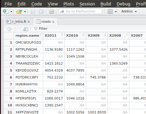
At this point, I will point out that the column names have been changed from the original CSV. Region name has become region.name and 2011 has become X2011. R uses the column header names as variables, so the column names need to be changed to proper variables names. It is possible to change the column names that R uses with the colnames() function, though I will keep the names that R assigned.

Note

In R, the . character is valid as a part of a variable name, so long as it is followed by a letter. Variables in R often contain . characters to separate words.

R vectors

Vectors in R are analogous to Python lists - they are a data structure that contains an ordered list of values. A vector can be created using the following syntax:

vector <- c(<element1>, <element2>, <element3>)

Try entering the following in your R console:

> c(1,2,3,4,5,6)

It is also possible to create a vector consisting of a sequence of numbers using the following syntax:

sequence_of_numbers <- <start_number>:<finish_number>

Try entering the following into your R console:

> 1:5

Vectors can be indexed using integer numbers or other vectors. For example, the following creates a vector called my.vector, prints the third value of my.vector, and then prints the first five values of my.vector:

my.vector=1:10
print(my.vector)
print(my.vector[3])
print(my.vector[1:5])

Note

Indexing in R starts with 1, so be sure not to get this mixed up with Python indexing, which starts at 0.

Indexing R dataframes

Individual columns can be selected from a dataframe using the $ symbol. The following selects the data from 2011 from the roads dataframe:

roads.2011 = roads$X2011

The resulting value is an R vector containing the values of the selected column. 

Dataframes can also be indexed by row and column using the following syntax:

new.dataframe <- original.dataframe[<row_index>,<column index>].

To select all rows or all columns, the row_index or column_index can be left blank. For example:

the.same.thing <- roads[,]

The rows and columns indices can both be an integer value or a vector of integer values. For example:

first.three.rows <- roads[1:3,]
first.three.columns <- roads[,1:3]

Row and column indices can also be a vector of logical values, as I will demonstrate later. Finally, the column index can be a vector of column names. For example:

X2011.with.region <- roads[,c("region.name","X2011")] 

In the next section, I'll show you how to use the tools that I've demonstrated so far to perform the task from Chapter 4, Reading, Analyzing, Modifying, and Writing Data - Part II, of finding the 2011 total road length.

Finding the 2011 total in R

Let's revisit the task of finding the 2011 total, this time using R. The first step is to extract the X2011 values. This has already been done in a previous step, which created the roads.2011 vector.

The next step is to find the sum of all of the values in the roads.2011 vector. One easy way is to use the built in R sum() function with a parameter that skips over NA values. I will show how to use the sum() function in this way this section (feel free to skip ahead if you want the short cut). 

First however, I will take a more round about approach to demonstrate the use of indexing. This will involve removing the NA values manually from the roads.2011 vector and then applying the sum() function.

You can create a vector of logical values using the is.na() function. The is.na() function takes as an argument a vector or dataframe and returns a vector or dataframe, respectively, of TRUE or FALSE values indicating whether the value of a position is NA. For example, you can try entering the following into the console:

> is.na(c(1,NA,2,NA,NA,3,4,NA,5))

You can create a vector of logical values corresponding to the NA values of roads.2011 using the is.na() function. The resulting vector can then be used to index and extract the non-NA values of the roads.2011 vector.

In the following line, a vector called not.na is created. The resulting not.na vector is a vector of logical values in which TRUE corresponds to an index of roads.2011 which is not NA and FALSE corresponds to an index of roads.2011 which is NA. The ! symbol is used to flip the TRUE and FALSE values so that TRUE corresponds to non-NA values.

not.na <- !is.na(total.2011)

Using an array of logical values to index a vector or a dataframe will extract all of the indices corresponding to a TRUE value. The following line will create a vector of all of the non-NA values in the roads.2011 vector:

roads.2011.cleaned <- roads.2011[not.na]TRUE and FALSE values so that TRUE corresponds to non-NA values._

Finally, the sum() function can be used to add the values:

total.2011<-sum(roads.2011.cleaned)

The more concise way of finding the sum is to set the na.rm of the sum function to TRUE, so that the function will skip over the NA values:

total.2011<-sum(roads.2011, na.rm=TRUE)

From the beginning, the following is the sequence of steps that have been used to read the data and find the 2011 total:

####
####
## reading in data
## set the working directory
## the working directory here should be changed 
## for your setup
setwd("path/to/your/project/folder")

## Read in the data, and assign to the roads_by_country
## variable. Roads by country is an R Dataframe
roads <- read.csv("data/artificial_roads_by_region.csv")

## select the 2011 column from the roads dataframe
roads.2011 <- roads$X2011

####
####
## finding the 2011 total

## create a index corresponding to not na values
not.na <- !is.na(roads.2011)

## index roads.2011 using not na
roads.2011.cleaned <- roads.2011[not.na]

## print the sum of the available roads in 2011.
total.2011<-sum(roads.2011.cleaned)

## the more concise way
total.2011<-sum(roads.2011, na.rm=TRUE)

Finding the sum of a column is a useful exercise in data manipulation; however, it may not be enough to get an accurate estimate, particularly if there is a high number of missing or erroneous values. (I created this particular dataset, so I can assure you that there are a number of missing and erroneous values.) In the following sections, I will go over some common techniques to clean numerical data. This will help to get more accurate results for the 2011 total, but it will also demonstrate some additional features of R and RStudio.

Before I get into the numerical data cleaning process, I will warn you that the variable names can get confusing, because there are several layers of filtering that take place. It is hard to represent all of these layers with a descriptive variable naming convention. The dplyr package, which I will introduce in the next chapter, will help considerably to keep R code concise and descriptive. For now, you can refer to a list of all of the variable names and their content at the end of the chapter.