Conducting basic outlier detection and removal

Outlier detection is a field of study in its own right, and deals with the detection of data that does not fit in a particular dataset. Advanced outlier detection techniques can be considered a part of data wrangling, but often draw from other fields, such as statistics and machine learning. For the purposes of this book, I will conduct a very basic form of outlier detection to find values that are too high. Values that are too high might be aggregates of the data or might reflect erroneous entries. 

In these next few steps, you will use the built-in plotting functionality in R to observe the data and look for particularly high values. 

The first step is to put the data in a form that can be easily visualized. A simple technique to capture the trend in the data by row is to find the means of all of the non-NA values in each data entry. This can be done using the rowMeans() function in R.

Before using the roawMeans() function, you will need to remove all of the non-numerical features - in this case, the region.name column. It is possible to index all of the columns except for one, by including a - sign before the index. The following creates a new dataframe without the region.name column:

roads.num <- roads[,-1]

The num in the roads.num dataframe stands for numerical because the roads.num dataframe just contains the numerical data.

With the first column removed, you can use the rowMeans function to obtain a vector with the mean value of each row. Like the sum() function, the rowMeans() function accepts an  na.rm parameter which will cause the function to ignore NA values. The following returns a vector with the mean value across each row:

roads.means <- rowMeans( roads.num , na.rm=TRUE )

To get a sense for how the data is distributed, you can plot a histogram of the means by using the hist() function as follows:

hist(roads.means)

In the lower right-hand corner of RStudio, you should see a histogram that is quite skewed towards the left. The following is the output on my computer:

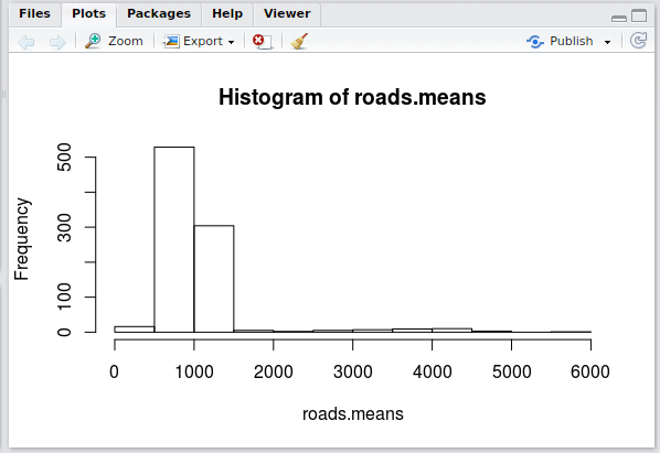
There appears to be a small number of values that are far to the right of the central distribution. Deciding what should be removed should usually be justified based on the particular project and the context of the data.

However, since this particular dataset doesn't quite have a context (it was randomly generated), I will remove the data that doesn't follow the general trend. The main distribution seems to go from zero to about 0 to 2000, so I will remove all of the rows with a mean greater than 2000.

To remove the rows whose means are greater than 2000, you can first create an index vector of logical values corresponding to row means less than 2000 as follows:

roads.keep <- roads.means < 2000

Finally, you can use the logical vector from the previous step to index the original roads dataframe. The following removes all of the rows with means greater than 2000:

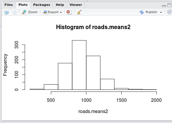
## remove entries with means greater than 2000
roads.keep <- roads.means < 2000

## remove outliers from the original dataframe 
roads2<-roads[roads.keep,]

## remove outliers from the numerical roads dataframe
roads.num2 <- roads.num[roads.keep,]

## remove outliers from the vector of means
## (we will use this later)
roads.means2 <- roads.means[roads.keep]

## plot the means with outliers removed
hist(roads.means2)

Plotting a histogram of the filtered row means now yields a recognizable normal distribution:

Now that the erroneous values are removed, the next step is to handle the missing values.