Deep learning is a subset of machine learning, which is a field of artificial intelligence that uses mathematics and computers to learn from data and map it from some input to some output. Loosely speaking, a map or a model is a function with parameters that maps the input to an output. Learning the map, also known as mode, occurs by updating the parameters of the map such that some expected empirical loss is minimized. The empirical loss is a measure of distance between the values predicted by the model and the target values given the empirical data.

Notice that this learning setup is extremely powerful because it does not require having an explicit understanding of the rules that define the map. An interesting aspect of this setup is that it does not guarantee that you will learn the exact map that maps the input to the output, but some other maps, as expected, predict the correct output.

This learning setup, however, does not come without a price: some deep learning methods require large amounts of data, specially when compared with methods that rely on feature engineering. Fortunately, there is a large availability of free data, specially unlabeled, in many domains.

Meanwhile, the term deep learning refers to the use of multiple layers in an ANN to form a deep chain of functions. The term ANN suggests that such models informally draw inspiration from theoretical models of how learning could happen in the brain. ANNs, also referred to as deep neural networks, are the main class of models considered in this book.

Despite its recent success in many applications, deep learning is not new and according to Ian Goodfellow, Yoshua Bengio, and Aaron Courville, there have been three eras:

• Cybernetics between the 1940s and the 1960s
• Connectionism between the 1980s and the 1990s
• The current deep learning renaissance beginning in 2006

Mathematically speaking, a neural network is a graph consisting of non-linear equations whose parameters can be estimated using methods such as stochastic gradient descent and backpropagation. We will introduce ANNs step by step, starting with linear and logistic regression.

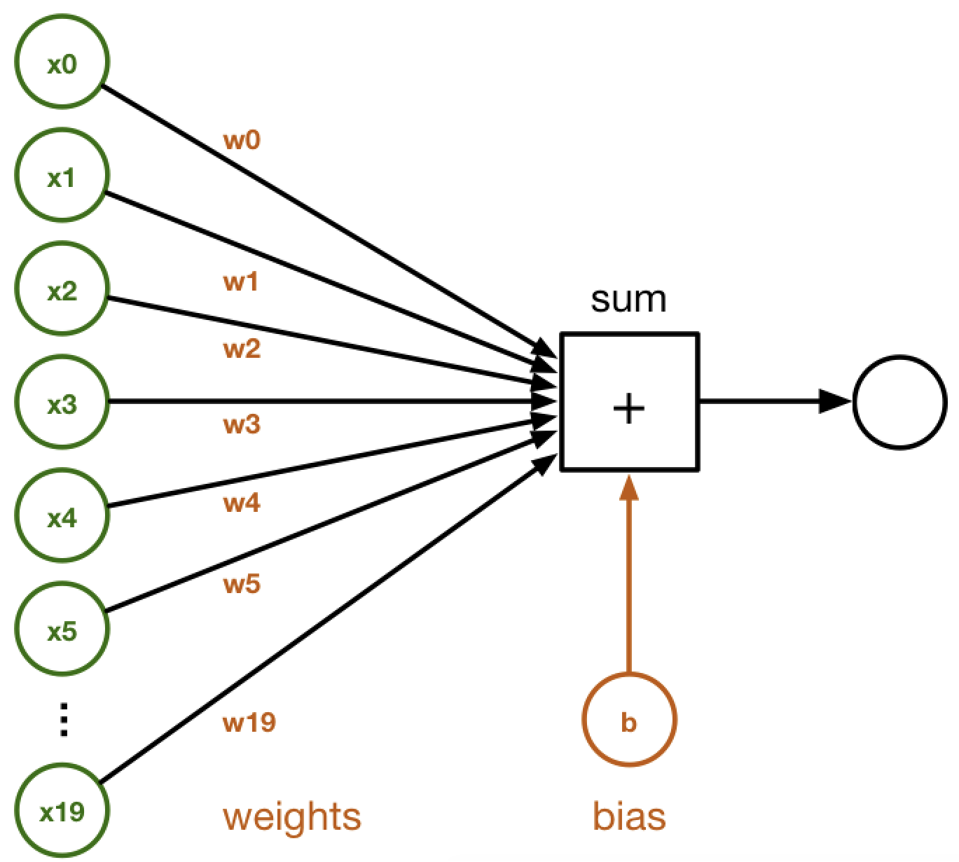
Linear regression is used to estimate the parameters of a model to describe the relationship between an output variable and the given input variables. It can be mathematically described as a weighted sum of input variables:

Here, the weight, , and inputs, , are vectors in ; in other words, they are real-valued vectors with dimensions, as a scalar bias term, and as a scalar term that represents the valuation of the function at the input  . In ANNs, the output of a single neuron without non-linearities is similar to the output of the linear model described in the preceding linear regression equation and the following diagram:

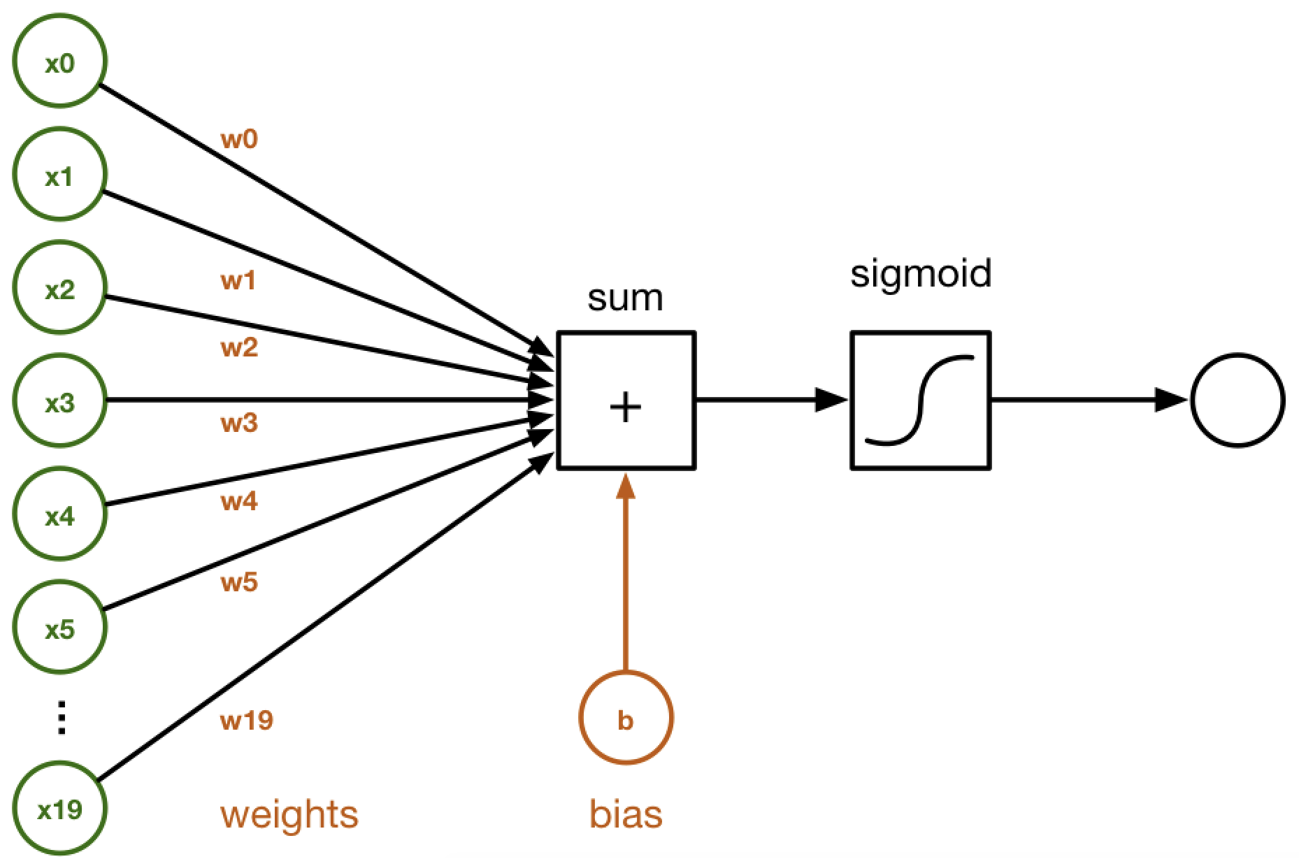
Logistic regression is a special version of regression where a specific non-linear function, the sigmoid function, is applied to the output of the linear model in the earlier linear regression equation:

The In ANNs, the non-linear model described in the logistic regression equation is similar to the output of a single neuron with a sigmoid non-linearity in the following diagram:

A combination of such neurons defines a hidden layer in a neural network, and the neural networks are organized as a chain of layers. The output of a hidden layer is described by the following equation and diagram:

Here, the weight, , and the input, , are vectors in _; is a scalar bias term, is a vector, and is a non-linearity:

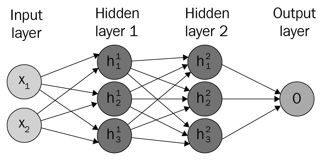
The preceding diagram depicts a fully connected neural network with two inputs, two hidden layers with three nodes each, and one output node.

In general, neural networks have a chain-like structure that is easy to visualize in equation form or as a graph, as the previous diagram confirms. For example, consider the and functions that are used in the model. In this simple model of a neural network, the input   is used to produce the output  ; the output of is used as the input of that finally produces .

In this simple model, the function   is considered to be the first hidden layer and the function   is considered to be the second hidden layer. These layers are called hidden because, unlike the input and the output values of the model that are known a priori, their values are not known.

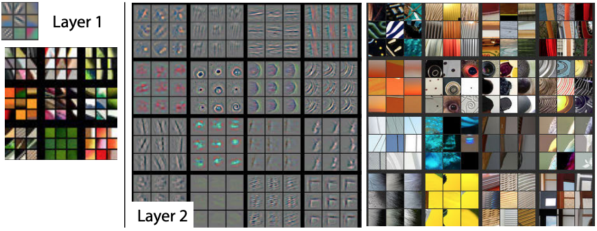
In each layer, the network is learning features or projections of the data that are useful for the task at hand. For example, in computer vision, there is evidence that the layers of the network closer to the input can learn filters that are associated with basic shapes, whereas in the layers closer to the output the network might learn filters that are closer to images.

The following figure taken from the paper Visualizing and Understanding Convolutional Networks by Zeiler et Fergus, provides a visualization of the filters on the first convolution layer of a trained AlexNet:

The output of each layer on the network is dependent on the parameters of the model estimated by training the neural network to minimize the loss with respect to the weights, , as we described earlier. This is a general principle in machine learning, in which a learning procedure, for example backpropagation, uses the gradients of the error of a model to update its parameters to minimize the error. Consider estimating the parameters of a linear regression model such that the output of the model minimizes the mean squared error (MSE). Mathematically speaking, the point-wise error between the predictions and the target value is computed as follows:

The MSE is computed as follows:

,

where presents the sum of the squared errors (SSE) and normalizes the SSE with the number of samples to reach the mean squared error (MSE).

In the case of linear regression, the problem is convex and the MSE has the simple closed solution given in the following equation:

Here, is the coefficient of the linear model, refers to matrices with the observations and their respective features, and is the response value associated with each observation. Note that this closed form solution requires the matrix to be invertible and, hence, to have a determinant larger than 0.

In the case of models where a closed solution to the loss does not exist, we can estimate the parameters that minimize the MSE by computing the partial derivative of each weight with respect to the MSE loss, , and using the negative of that value, scaled by a learning rate, , to update the parameters of the model being evaluated:

A model in which many of the coefficients in are 0 is said to be sparse. Given the large number of parameters or coefficients in deep learning models, producing models that are sparse is valuable because it can reduce computation requirements and produce models with faster inference.

The backpropagation algorithm is a special case of reverse-mode automatic differentiation. In its basic modern version, the backpropagation algorithm has become the standard for training neural networks, possibly due to its underlying simplicity and relative power.

Inspired by the work of Donal Hebb and the so-called Hebb rule, Rosenblatt developed the idea of a perceptron that was based on the formation and changes of synapses between neurons, where the output of a neuron will be modeled as a weighted sum based on its incoming signals. This weighted sum is similar to what we described in the equation(3) in this chapter.

The basic idea of backpropagation is as follows: to define an error function and reiteratively compute the gradients of the loss with respect to the model weights and perform gradient descent and weight updates that are optimal for minimizing the error function given the current data and model weights. From a perspective of calculus, backpropagation is an algorithm that efficiently computes the chain rule with a specific order of operations.

The data and the error function are extremely important factors of the learning procedure. For example, consider a classifier that is trained to identify single handwritten digits. For training the model, suppose we will use the MNIST dataset, (http://yann.lecun.com/exdb/mnist/) which is comprises 28 by 28 monochromatic images of single handwritten white digits on a black canvas, such as the ones in following figure. Ideally, we want the model to predict 1 whenever the image looks such as a 1, 2 whenever it looks such as a 2, and so on:

Note that backpropagation does not define what aspects of the images should be considered, nor does it provide guarantees that the classifier will not memorize the data or that it will get generalize to unseen examples. A model trained with such data will fail if the colors are inverted, for instance, black digits on a white canvas. Naturally, one way to fix this issue will be to augment the data to include images with any foreground and background color combination. This example illustrates the importance of the training data and the objective function being used.

A loss function, also known as a cost function, is a function that maps an event or values of one or more variables onto a real number intuitively representing some cost associated with the event. We will cover the following three loss functions in this chapter:

• L1 Loss
• L2 Loss
• Categorical Crossentropy Loss

The L1 loss function, also known as the mean absolute error, measures the average point-wise difference between the model prediction, , and the target value, . The partial derivative is equal to 1 when the model prediction is larger than the target value, and equal to -1 when the prediction is smaller than the target error. This property of the L1 loss function can be used to circumvent problems that might arise when learning from noisy labels:

The L2 loss function, also known as MSE, measures the average point-wise squared difference between the prediction, , and the target value, . Compared to the L1 loss function, the L2 loss function penalizes larger errors:

The categorical crossentropy loss function measures the weighted divergence between targets, , and predictions, , where denotes the data point, and denotes the class. For single label classification problems, the targets operate as an indicator variable and the loss is reduced to :

ANNs are normally non-linear models that use different types of non-linearities. The most commonly used are as follows:

• sigmoid
• Tanh
• ReLU

The sigmoid non-linearity has an S shape and maps the input domain to an output range between [0, 1]. This characteristic of sigmoid makes it suitable for estimating probabilities, which are also in the [0, 1] range. The gradient of sigmoid is larger at its center, 0.0, and the gradients quickly vanish as the domain moves away from 0.0:

The Tanh non-linearity has an S shape that is similar to the sigmoid non-linearity, but maps the input domain to an output range between [-1, 1]. In the same way as sigmoid, the gradient of Tanh is larger at its center, 0.0, but the gradient at the center is larger for the Tanh non-linearity, hence the derivatives are steeper and the gradient is stronger:

The ReLU non-linearity is a piecewise linear function with a non-linearity introduced by rectification. Unlike the sigmoid and Tanh non-linearities that have continuous gradients, the gradients of ReLU have two values only: 0 for values smaller than 0, and 1 for values larger than 0. Hence, the gradients of ReLU are sparse. Although the gradient of ReLU at 0 is undefined, common practice sets it to 0. There are variations to the ReLU non-linearity including the ELU and the Leaky RELU. Compared to sigmoid and Tanh, the derivative of ReLU is faster to compute and induces sparsity in models:

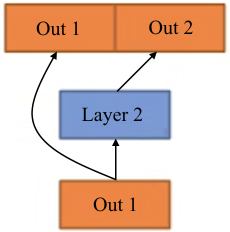
Feedforward neural networks have this name because the flow of information being evaluated by the neural network starts at the input  , flows all the way through the hidden layers, and finally reaches the output  . Note that the output of each layer does flow back to itself. In some models there are residual connections in which the input of the layer is added or concatenated to the output of the layer itself. In the following figure, we provide a visualization in which the input of Layer 2, Out 1, is concatenated with the output of Layer 2:

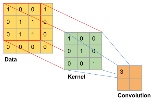
Convolutional Neural Networks (CNNs) are neural networks that learn filters, tensors in , which are convolved with the data. In the image domain, a filter is usually square and with small sizes ranging from 3 x 3 to 9 x 9 in pixel size. The convolution operation can be interpreted as sliding a filter over the data and, for each position, applying a dot product between the filter and the data at that position. The following diagram shows an intermediary step of convolution with stride 1 where the kernel in green is convolved with the first area in the data, represented by the red grid:

A special characteristic of CNNs is that the weights of the filters are learned. For example, if the task at hand is classifying monochromatic handwritten digits from the MNIST dataset, the ANN might learn filters that look similar to vertical, horizontal, and diagonal lines.

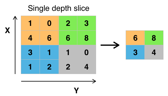
The max pooling layer is a common non-linear filter in computer vision applications. Given an by window, it consists of choosing the largest value in that window. The max pooling layers reduces the dimensionality of the data, potentially preventing overfitting and reducing computational cost. Given that within the window the max pooling layer takes the largest value in the window, disregarding spatial information, the max pooling layers can be used to learn the representations that are locally invariant to translation:

In this section, we will provide instructions on how to set up a Python deep learning programming environment that will be used throughout the book. We will start with Anaconda, which makes package management and deployment easy, and NVIDIA's CUDA Toolkit and cuDNN, which make training and inference in deep learning models quick. There are several compute cloud services, like Amazon Web Services (AWS), that provide ready to use deep learning environments with NVIDIA GPUs.

Anaconda is a free and open source efficient distribution that provides easy package management and deployment for the programming languages R and Python. Anaconda focuses on data science and deep learning applications and provides over 6 million users with hundreds of packages and support for Windows, Linux, and macOS.

Installing Anaconda is easy and simply requires downloading the installation wizard for a target Python version. We are going to download Anaconda's installation wizard for Python 3.5. The installation wizard can be downloaded on Anaconda's website at https://www.anaconda.com/download/.

After following the wizard instructions and installing Anaconda, we are going to update all Anaconda packages using the conda command. To do so, open Anaconda's Command-Line Interface (CLI) and type the following commands:

conda update conda
conda update –all

A virtual environment allows us to have different versions of libraries and executables, avoiding conflicts between them and making it easy to develop multiple projects at the same time. Creating a virtual environment in Anaconda is easy and only requires executing a single command on Anaconda's CLI. With the following command, we are going to create a virtual environment running Python 3.5 and name it deeplearning:

conda create -n deeplearning pip python=3.5

Now that we have created the deeplearning virtual environment, we are going to activate it so that we can start populating it with Python packages. To do so, open Anaconda's CLI and type the following command:

activate deeplearning

After typing this command, your CLI prompt should change and include a prefix to indicate that the virtual environment is currently active.

TensorFlow is a high-level deep learning API written in Python and developed by Google. In this book, TensorFlow will be the backend that supports Keras, our main deep learning API. Follow instructions on the following website: https://www.tensorflow.org/install/install_linux#tensorflow_gpu_support. Choose your OS, and install TensorFlow for Python 3.5 with GPU support.

Keras is a high-level deep learning API written in Python that supports TensorFlow, CNTK, and Theano as backends. Keras has the main building blocks for building, training, and prototyping deep learning projects. The building blocks in Keras include neural network layers, optimization functions, activation functions, and several tools for working with data and training in general.

Installing keras is easy! Inside our deeplearning virtual environment, type the following command:

pip install keras

In addition to Keras, the main deep learning library used in this book, we are going to install libraries for data visualization and machine learning in general. These libraries provide valuable tools to help developers easily build training pipelines, evaluate and train models more efficiently, and visualize data quickly and effortlessly.

Although there are distributions like Anaconda that provide environments with such libraries already installed by default, we describe the installation procedures here such that the reader learns the process and does not become dependent on pre-packaged third party distributions.

The most widely used data visualization library in Python is called matplotlib. It enables the quick and easy creation of publication-quality complex plots and graphs, which facilitate understanding data. Matploblib can be installed with pip as follows:

pip install matplotlib

Jupyter is another widely used and valuable Python library. It includes Jupyter notebooks, which allow interactive and quick prototyping in Python and other languages on the browser. Jupyter also supports data visualization, including images, video, and audio! Jupyter notebooks can be shared and accessed via a web browser. Jupyter can be installed with pip as follows:

pip install jupyter

Scikit-learn is the leading Python library for machine learning and data science in general. Scikit-learn is open source and built on top of NumPy, SciPy, and matplotlib. It contains a wide range of machine learning models and algorithms, including classification, regression, clustering, dimensionality reduction, model selection, data preprocessing, metrics, and many other valuable things. Scikit-learn can be installed with pip as follows:

pip install sklearn

Now that we have installed our libraries, it is time to make sure everything works as expected.

NVIDIA's CUDA Toolkit provides a development environment for creating high-performance GPU-accelerated applications. You can develop, optimize, and deploy your applications on GPU-accelerated embedded systems, workstations, enterprise data centers, cloud-based platforms, and HPC supercomputers using the CUDA Toolkit. The Toolkit includes GPU-accelerated libraries, debugging and optimization tools, a C/C++ compiler, and a runtime library to deploy your application.

NVIDIA's cuDNN is a GPU-accelerated library of primitives for deep neural networks. cuDNN provides highly-tuned implementations for standard routines such as forward and backward convolution, pooling, normalization, and activation layers. cuDNN is part of the NVIDIA Deep Learning SDK.

cuDNN is available for members of the NVIDIA Developer Program. Registration to this program is free and members are given access to the latest NVIDIA SDKs and tools to accelerate building applications in key technology areas such as artificial intelligence, deep learning, accelerated computing, and advanced graphics (https://developer.nvidia.com/rdp/cudnn-download).

Now that we have installed NVIDIA's CUDA Toolkit and NVIDIA's cuDNN, our next step is to add environment paths.

We are going to verify our deep learning environment installation by building and training a simple fully-connected neural network to perform classification on images of handwritten digits from the MNIST dataset. MNIST is an introductory dataset that contains 70,000 images, thus enabling us to quickly train a small model on a CPU and extremely fast on the GPU. In this simple example, we are only interested in testing our deep learning setup.

We start by using the keras built-in function to download and load the train and test datasets associated with MNIST:

import numpy as np
from keras.datasets import mnist
from keras.models import Sequential
from keras.utils import np_utils
from keras.optimizers import SGD
from keras.layers.core import Dense,Activation

The training set has 60,000 samples and the test set has 10,000 samples. The dataset is balanced and shuffled, that is, it has a similar number of samples for each class and the orders of the samples are random:

(X_train, y_train), (X_test, y_test) = mnist.load_data()
print("Train samples {}, Train labels {}".format(X_train.shape, y_train.shape))
print("Test samples {}, Test labels {}".format(X_test.shape, y_test.shape))

The MNIST dataset contains images of 28 by 28. To train our dense neural network, we need to combine the height and width dimensions of the image to make it unidimensional, while keeping the same batch size, that is, the number of items in the batch. After reshaping the data, we will convert it to floating point and scale it to [-1, 1] following neural networks tricks of the trade described in Yann Lecun's Efficient Backprop paper:

# reshape to batch size by height * width
h, w = X_train.shape[1:]
X_train = X_train.reshape(X_train.shape[0], h * w)
X_test = X_test.reshape(X_test.shape[0], h * w)
X_train = X_train.astype('float32')
X_test = X_test.astype('float32')
# scale to [0, 1], scale to [0, 2], offset by -1
X_train = (X_train / 255.0) * 2 - 1
X_test = (X_test - 255.0) * 2 - 1

For training our network, Keras requires each of our image labels to be in the one-hot representation. In the one-hot representation, we have a vector whose length is equal to the number of classes in which the index that represented the class associated with that label is 1, and 0 otherwise:

# convert class vectors to a matrix of one-hot vectors
n_classes = 10
y_train = np_utils.to_categorical(y_train, n_classes)
y_test = np_utils.to_categorical(y_test, n_classes)

After having prepared the data, we will define the parameters of our model and instantiate it. We now import from Keras the functions that are necessary to building and training a fully connected neural network. Whereas the Dense class instantiates a dense layer, the Sequential class allows us to connect these Dense layers in a chain. Lastly, we import the Stochastic Gradient Descent optimizer such that we can perform gradient descent on the loss given to the model to update the model parameters. We create a model with two hidden layers. The first layer projects the reshaped h * w image input to 128 nodes, and the second layer projects the 128 nodes down to 10 nodes representing the number of classes in this problem:

n_hidden = 128
model = Sequential()
model.add(Dense(n_hidden, activation='tanh', input_dim=h*w))
model.add(Dense(n_classes, activation='softmax'))
model.summary()

After defining our model, we define the optimizer's parameters that will be used to update the weights of our model given the loss. We choose a small learning of 0.001 and use the defaults for the other parameters:

sgd = SGD(lr=0.001)

Finally, we compile the graph of our model setting the loss function to categorical_crossentropy, which is used in classification problems where each sample belongs to a single class. We use accuracy as the reported metric because for this problem we are interested in increasing the accuracy metric of our model:

model.compile(loss='categorical_crossentropy', optimizer=sgd, metrics=['accuracy'])

We train our model for as many epochs as necessary. One epoch is equivalent to a pass through the entire training data. The batch size is chosen such that it maximizes memory performance by maxing out memory footprint during training. This is very important, especially when using GPUs, such that our models use all the resources available in parallel:

model.fit(X_train, y_train, epochs=10, batch_size=128)

After training the model, we can check whether our model is generalizing to data that it has not seen by looking at our model's performance on the test data:

score = model.evaluate(X_test, y_test, batch_size=128)
print(score)

The preceding code block generates the following output:

In this chapter, we covered essential knowledge for building and training deep learning models, starting with a simple example based on linear regression. We covered important topics in machine learning such as parameter estimation and backpropagation, loss functions, and diverse neural network layers. We described how to set up a deep learning programming environment that will be used throughout this book. After installing our deep learning programming environment, we trained and evaluated a simple neural network model for the classification of handwritten digits.

In the next chapter, we will cover generative models, explaining the advantages and disadvantages of each class of generative models, including GANs.