The theoretical foundations of RL
In this section, I will introduce you to the mathematical representation and notation of the formalisms (reward, agent, actions, observations, and environment) that we just discussed. Then, using this as a knowledge base, we will explore the second-order notions of the RL language, including state, episode, history, value, and gain, which will be used repeatedly to describe different methods later in the book.
Markov decision processes
Before that, we will cover Markov decision processes (MDPs), which will be described like a Russian matryoshka doll: we will start from the simplest case of a Markov process (MP), then extend that with rewards, which will turn it into a Markov reward process. Then, we will put this idea into an extra envelope by adding actions, which will lead us to an MDP.
MPs and MDPs are widely used in computer science and other engineering fields. So, reading this chapter will be useful for you not only for RL contexts, but also for a much wider range of topics. If you're already familiar with MDPs, then you can quickly skim this chapter, paying attention only to the terminology definitions, as we will use them later on.
The Markov process
Let's start with the simplest child of the Markov family: the MP, which is also known as the Markov chain. Imagine that you have some system in front of you that you can only observe. What you observe is called states, and the system can switch between states according to some laws of dynamics. Again, you cannot influence the system, but can only watch the states changing.
All possible states for a system form a set called the state space. For MPs, we require this set of states to be finite (but it can be extremely large to compensate for this limitation). Your observations form a sequence of states or a chain (that's why MPs are also called Markov chains). For example, looking at the simplest model of the weather in some city, we can observe the current day as sunny or rainy, which is our state space. A sequence of observations over time forms a chain of states, such as [sunny, sunny, rainy, sunny, …], and this is called history.
To call such a system an MP, it needs to fulfill the Markov property, which means that the future system dynamics from any state have to depend on this state only. The main point of the Markov property is to make every observable state self-contained to describe the future of the system. In other words, the Markov property requires the states of the system to be distinguishable from each other and unique. In this case, only one state is required to model the future dynamics of the system and not the whole history or, say, the last N states.
In the case of our toy weather example, the Markov property limits our model to represent only the cases when a sunny day can be followed by a rainy one with the same probability, regardless of the amount of sunny days we've seen in the past. It's not a very realistic model, as from common sense we know that the chance of rain tomorrow depends not only on the current conditions but on a large number of other factors, such as the season, our latitude, and the presence of mountains and sea nearby. It was recently proven that even solar activity has a major influence on the weather. So, our example is really naïve, but it's important to understand the limitations and make conscious decisions about them.
Of course, if we want to make our model more complex, we can always do this by extending our state space, which will allow us to capture more dependencies in the model at the cost of a larger state space. For example, if you want to capture separately the probability of rainy days during summer and winter, then you can include the season in your state.
In this case, your state space will be [sunny+summer, sunny+winter, rainy+summer, rainy+winter] and so on.
As your system model complies with the Markov property, you can capture transition probabilities with a transition matrix, which is a square matrix of the size N×N, where N is the number of states in our model. Every cell in a row, i, and a column, j, in the matrix contains the probability of the system to transition from state i to state j.
For example, in our sunny/rainy example, the transition matrix could be as follows:
| Sunny | Rainy | |
|
Sunny |
0.8 |
0.2 |
|
Rainy |
0.1 |
0.9 |
In this case, if we have a sunny day, then there is an 80% chance that the next day will be sunny and a 20% chance that the next day will be rainy. If we observe a rainy day, then there is a 10% probability that the weather will become better and a 90% probability of the next day being rainy.
So, that's it. The formal definition of an MP is as follows:
- A set of states (S) that a system can be in
- A transition matrix (T), with transition probabilities, which defines the system dynamics
A useful visual representation of an MP is a graph with nodes corresponding to system states and edges, labeled with probabilities representing a possible transition from state to state. If the probability of a transition is 0, we don't draw an edge (there is no way to go from one state to another). This kind of representation is also widely used in finite state machine representation, which is studied in automata theory.
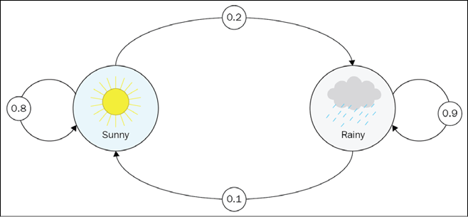
Figure 1.4: The sunny/rainy weather model
Again, we're talking about observation only. There is no way for us to influence the weather, so we just observe it and record our observations.
To give you a more complicated example, let's consider another model called office worker (Dilbert, the main character in Scott Adams' famous cartoons, is a good example). His state space in our example has the following states:
- Home: He's not at the office
- Computer: He's working on his computer at the office
- Coffee: He's drinking coffee at the office
- Chatting: He's discussing something with colleagues at the office
The state transition graph looks like this:
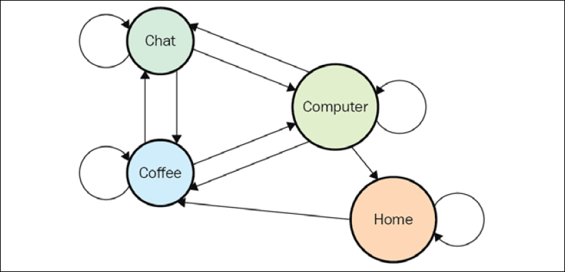
Figure 1.5: The state transition graph for our office worker
We assume that our office worker's weekday usually starts from the Home state and that he starts his day with Coffee without exception (no  edge and no
  edge). The preceding diagram also shows that workdays always end (that is, going to the Home state) from the Computer state.
The transition matrix for the preceding diagram is as follows:
| Home | Coffee | Chat | Computer | |
| Home |
60% |
40% |
0% |
0% |
| Coffee |
0% |
10% |
70% |
20% |
| Chat |
0% |
20% |
50% |
30% |
| Computer |
20% |
20% |
10% |
50% |
The transition probabilities could be placed directly on the state transition graph, as shown here:
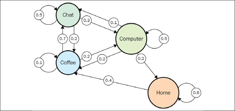
Figure 1.6: The state transition graph with transition probabilities
In practice, we rarely have the luxury of knowing the exact transition matrix. A much more real-world situation is when we only have observations of our system's states, which are also called episodes:


It's not complicated to estimate the transition matrix from our observations—we just count all the transitions from every state and normalize them to a sum of 1. The more observation data we have, the closer our estimation will be to the true underlying model.
It's also worth noting that the Markov property implies stationarity (that is, the underlying transition distribution for any state does not change over time). Nonstationarity means that there is some hidden factor that influences our system dynamics, and this factor is not included in observations. However, this contradicts the Markov property, which requires the underlying probability distribution to be the same for the same state regardless of the transition history.
It's important to understand the difference between the actual transitions observed in an episode and the underlying distribution given in the transition matrix. Concrete episodes that we observe are randomly sampled from the distribution of the model, so they can differ from episode to episode. However, the probability of the concrete transition to be sampled remains the same. If this is not the case, Markov chain formalism becomes nonapplicable.
Now we can go further and extend the MP model to make it closer to our RL problems. Let's add rewards to the picture!
Markov reward processes
To introduce reward, we need to extend our MP model a bit. First, we need to add value to our transition from state to state. We already have probability, but probability is being used to capture the dynamics of the system, so now we have an extra scalar number without extra burden.
Reward can be represented in various forms. The most general way is to have another square matrix, similar to the transition matrix, with reward given for transitioning from state i to state j, which reside in row i and column j.
As mentioned, reward can be positive or negative, large or small. In some cases, this representation is redundant and can be simplified. For example, if reward is given for reaching the state regardless of the previous state, we can keep only 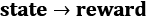 pairs, which are a more compact representation. However, this is applicable only if the reward value depends solely on the target state, which is not always the case.
The second thing we're adding to the model is the discount factor  (gamma), which is a single number from 0 to 1 (inclusive). The meaning of this will be explained after the extra characteristics of our Markov reward process have been defined.
As you will remember, we observe a chain of state transitions in an MP. This is still the case for a Markov reward process, but for every transition, we have our extra quantity—reward. So now, all our observations have a reward value attached to every transition of the system.
For every episode, we define return at the time, t, as this quantity:
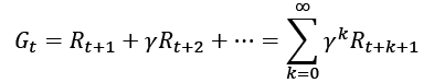
Let's try to understand what this means. For every time point, we calculate return as a sum of subsequent rewards, but more distant rewards are multiplied by the discount factor raised to the power of the number of steps we are away from the starting point at t. The discount factor stands for the foresightedness of the agent. If gamma equals 1, then return, Gt, just equals a sum of all subsequent rewards and corresponds to the agent that has perfect visibility of any subsequent rewards. If gamma equals 0, Gt will be just immediate reward without any subsequent state and will correspond to absolute short-sightedness.
These extreme values are useful only in corner cases, and most of the time, gamma is set to something in between, such as 0.9 or 0.99. In this case, we will look into future rewards, but not too far. The value of  might be applicable in situations of short finite episodes.
This gamma parameter is important in RL, and we will meet it a lot in the subsequent chapters. For now, think about it as a measure of how far into the future we look to estimate the future return. The closer it is to 1, the more steps ahead of us we will take into account.
This return quantity is not very useful in practice, as it was defined for every specific chain we observed from our Markov reward process, so it can vary widely, even for the same state. However, if we go to the extreme and calculate the mathematical expectation of return for any state (by averaging a large number of chains), we will get a much more useful quantity, which is called the value of the state:
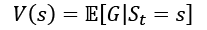
This interpretation is simple—for every state, s, the value, V(s), is the average (or expected) return we get by following the Markov reward process.
To show this theoretical stuff in practice, let's extend our office worker (Dilbert) process with reward and turn it into a Dilbert reward process (DRP). Our reward values will be as follows:
 (as it's good to be home)
 (working hard is a good thing)
 (it's not good to be distracted)
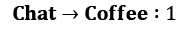
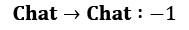 (long conversations become boring)
A diagram of this is shown here:
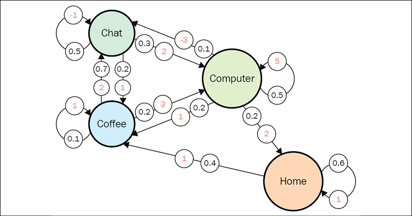
Figure 1.7: A state transition graph with transition probabilities (dark) and rewards (light)
Let's return to our gamma parameter and think about the values of states with different values of gamma. We will start with a simple case: gamma = 0. How do you calculate the values of states here? To answer this question, let's fix our state to Chat. What could the subsequent transition be? The answer is that it depends on chance. According to our transition matrix for the Dilbert process, there is a 50% probability that the next state will be Chat again, 20% that it will be Coffee, and 30% that it will be Computer. When gamma = 0, our return is equal only to a value of the next immediate state. So, if we want to calculate the value of the Chat state, then we need to sum all transition values and multiply that by their probabilities:
V(chat) = –1 * 0.5 + 2 * 0.3 + 1 * 0.2 = 0.3
V(coffee) = 2 * 0.7 + 1 * 0.1 + 3 * 0.2 = 2.1
V(home) = 1 * 0.6 + 1 * 0.4 = 1.0
V(computer) = 5 * 0.5 + (–3) * 0.1 + 1 * 0.2 + 2 * 0.2 = 2.8
So, Computer is the most valuable state to be in (if we care only about immediate reward), which is not surprising as  is frequent, has a large reward, and the ratio of interruptions is not too high.
Now a trickier question—what's the value when gamma = 1? Think about this carefully. The answer is that the value is infinite for all states. Our diagram doesn't contain sink states (states without outgoing transitions), and when our discount equals 1, we care about a potentially infinite number of transitions in the future. As you've seen in the case of gamma = 0, all our values are positive in the short term, so the sum of the infinite number of positive values will give us an infinite value, regardless of the starting state.
This infinite result shows us one of the reasons to introduce gamma into a Markov reward process instead of just summing all future rewards. In most cases, the process can have an infinite (or large) amount of transitions. As it is not very practical to deal with infinite values, we would like to limit the horizon we calculate values for. Gamma with a value less than 1 provides such a limitation, and we will discuss this later in this book. On the other hand, if you're dealing with finite-horizon environments (for example, the tic-tac-toe game, which is limited by at most nine steps), then it will be fine to use gamma = 1. As another example, there is an important class of environments with only one step called the multi-armed bandit MDP. This means that on every step, you need to make a selection of one alternative action, which provides you with some reward and the episode ends.
As I already mentioned about the Markov reward process, gamma is usually set to a value between 0 and 1. However, with such values, it becomes almost impossible to calculate them accurately by hand, even for Markov reward processes as small as our Dilbert example, because it will require summing hundreds of values. Computers are good at tedious tasks such as this, and there are several simple methods that can quickly calculate values for Markov reward processes for given transition and reward matrices. We will see and even implement one such method in Chapter 5, Tabular Learning and the Bellman Equation, when we will start looking at Q-learning methods.
For now, let's put another layer of complexity around our Markov reward processes and introduce the final missing piece: actions.
Adding actions
You may already have ideas about how to extend our Markov reward process to include actions. Firstly, we must add a set of actions (A), which has to be finite. This is our agent's action space. Secondly, we need to condition our transition matrix with actions, which basically means that our matrix needs an extra action dimension, which turns it into a cube.
If you remember, in the case of MPs and Markov reward processes, the transition matrix had a square form, with the source state in rows and target state in columns. So, every row, i, contained a list of probabilities to jump to every state:
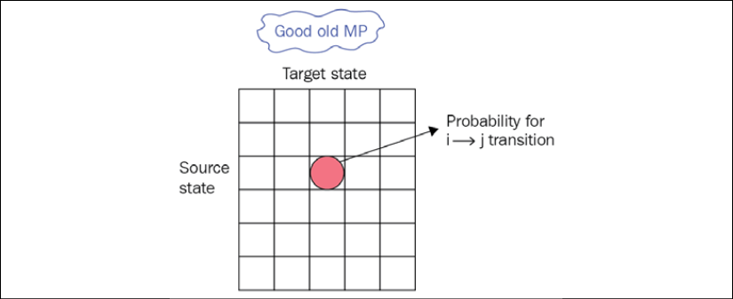
Figure 1.8: The transition matrix in square form
Now the agent no longer passively observes state transitions, but can actively choose an action to take at every state transition. So, for every source state, we don't have a list of numbers, but we have a matrix, where the depth dimension contains actions that the agent can take, and the other dimension is what the target state system will jump to after actions are performed by the agent. The following diagram shows our new transition table, which became a cube with the source state as the height dimension (indexed by i), the target state as the width (j), and the action the agent can take as the depth (k) of the transition table:
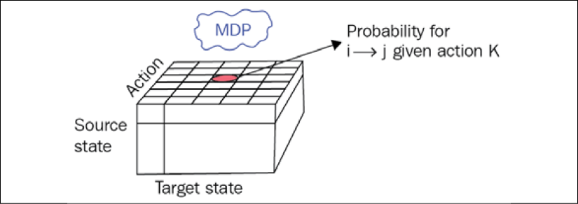
Figure 1.9: Transition probabilities for the MDP
So, in general, by choosing an action, the agent can affect the probabilities of the target states, which is a useful ability.
To give you an idea of why we need so many complications, let's imagine a small robot that lives in a 3×3 grid and can execute the actions turn left, turn right, and go forward. The state of the world is the robot's position plus orientation (up, down, left, and right), which gives us 3 × 3 × 4 = 36 states (the robot can be at any location in any orientation).
Also, imagine that the robot has imperfect motors (which is frequently the case in the real world), and when it executes turn left or turn right, there is a 90% chance that the desired turn happens, but sometimes, with a 10% probability, the wheel slips and the robot's position stays the same. The same happens with go forward—in 90% of cases it works, but for the rest (10%) the robot stays at the same position.
In the following illustration, a small part of a transition diagram is shown, displaying the possible transitions from the state (1, 1, up), when the robot is in the center of the grid and facing up. If the robot tries to move forward, there is a 90% chance that it will end up in the state (0, 1, up), but there is a 10% probability that the wheels will slip and the target position will remain (1, 1, up).
To properly capture all these details about the environment and possible reactions to the agent's actions, the general MDP has a 3D transition matrix with the dimensions source state, action, and target state.
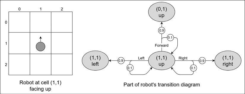
Figure 1.10: A grid world environment
Finally, to turn our Markov reward process into an MDP, we need to add actions to our reward matrix in the same way that we did with the transition matrix. Our reward matrix will depend not only on the state but also on the action. In other words, the reward the agent obtains will now depend not only on the state it ends up in but also on the action that leads to this state.
This is similar to when you put effort into something—you're usually gaining skills and knowledge, even if the result of your efforts wasn't too successful. So, the reward could be better if you're doing something rather than not doing something, even if the final result is the same.
Now, with a formally defined MDP, we're finally ready to cover the most important thing for MDPs and RL: policy.
Policy
The simple definition of policy is that it is some set of rules that controls the agent's behavior. Even for fairly simple environments, we can have a variety of policies. For example, in the preceding example with the robot in the grid world, the agent can have different policies, which will lead to different sets of visited states. For example, the robot can perform the following actions:
- Blindly move forward regardless of anything
- Try to go around obstacles by checking whether that previous forward action failed
- Funnily spin around to entertain its creator
- Choose an action by randomly modeling a drunk robot in the grid world scenario
You may remember that the main objective of the agent in RL is to gather as much return as possible. So, again, different policies can give us different amounts of return, which makes it important to find a good policy. This is why the notion of policy is important.
Formally, policy is defined as the probability distribution over actions for every possible state:
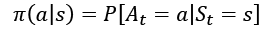
This is defined as probability and not as a concrete action to introduce randomness into an agent's behavior. We will talk later in the book about why this is important and useful. Deterministic policy is a special case of probabilistics with the needed action having 1 as its probability.
Another useful notion is that if our policy is fixed and not changing, then our MDP becomes a Markov reward process, as we can reduce the transition and reward matrices with a policy's probabilities and get rid of the action dimensions.
Congratulations on getting to this stage! This chapter was challenging, but it was important for understanding subsequent practical material. After two more introductory chapters about OpenAI Gym and deep learning, we will finally start tackling this question—how do we teach agents to solve practical tasks?