How-To Tutorials - Data

  MySQL for Python Integrate the flexibility of Python and the power of MySQL to boost the productivity of your Python applications Implement the outstanding features of Python's MySQL library to their full potential See how to make MySQL take the processing burden from your programs Learn how to employ Python with MySQL to power your websites and desktop applications Apply your knowledge of MySQL and Python to real-world problems instead of hypothetical scenarios A manual packed with step-by-step exercises to integrate your Python applications with the MySQL database server         Read more about this book       (For more resources on this subject, see here.) Objective: Install a C compiler on Windows installation. Tip: Windows binaries do not currently exist for the 1.2.3 version of MySQL for Python. To get them, you would need to install a C compiler on your Windows installation and compile the binary from source. Objective: Use tar.gz to use egg file. Tip: If you cannot use egg files or if you use an earlier version of Python, you should use the tar.gz file, a tar and gzip archive. The tar.gz archive follows the Linux egg files in the file listing. The current version of MySQL for Python is 1.2.3c1, so the file we want is as following: MySQL-python-1.2.3c1.tar.gz This method is by far more complicated than the others. If at all possible, use your operating system's installation method or an egg file. Objective: Limitation of using MySQL for Python on Python version. Tip: This version of MySQL for Python is compatible up to Python 2.6. It is worth noting that MySQL for Python has not yet been released for Python 3.0 or later versions. In your deployment of the library, therefore, ensure that you are running Python 2.6 or earlier. As noted, Python 2.5 and 2.6 have version-specifi c releases. Prior to Python 2.4, you will need to use either a tar.gz version of the latest release or use an older version of MySQL for Python. The latter option is not recommended. Objective: It is important to phrase the query in such a way as to narrow the returned values as much as possible. Tip: Here, instead of returning whole records, we tell MySQL to return only the namecolumn. This natural reduction in the data reduces processing time for both MySQL and Python. This saving is then passed on to your server in the form of more sessions able to be run at one time. Objective: This hard-wiring of the search query allows us to test the connection before coding the rest of the function. Tip: There may be a tendency here to insert user-determined variables immediately. With experience, it is possible to do this. However, if there are any doubts about the availability of the database, your best fallback position is to keep it simple and hardwired. This reduces the number of variables in making a connection and helps one to blackbox the situation, making troubleshooting much easier. Objective: Readability counts. Tip: The virtue of readability in programming is often couched in terms of being kind to the next developer who works on your code. There is more at stake, however. With readability comes not only maintainability but control. If it takes you too much effort to understand the code you have written, you will have a harder time controlling the program's flow and this will result in unintended behavior. The natural consequence of unintended program behavior is the compromising of process stability and system security. Objective: Quote marks not necessary when assigning MySQL statements. Tip: It is not necessary to use triple quote marks when assigning the MySQL sentence to statement or when passing it to execute(). However, if you used only a single pair of either double or single quotes, it would be necessary to escape every similar quote mark. As a stylistic rule, it is typically best to switch to verbatim mode with the triple quote marks in order to ensure the readability of your code. Objective: xrange() is much more memory efficient than range(). Tip: The differences between xrange() and range() are often overlooked or even ignored. Both count through the same values, but they do it differently. Where range() calculates a list the first time it is called and then stores it in memory, xrange() creates an immutable sequence that returns the next in the series each time it is called. As a consequence, xrange() is much more memory efficient than range(), especially when dealing with large groups of integers. As a consequence of its memory efficiency, however, it does not support functionality such as slicing, which range() does, because the series is not yet fully determined. Objective: autocommit feature is useful in MySQL for Python . Tip: Unless you are running several database threads at a time or have to deal with similar complexity, MySQL for Python does not require you to use either commit() or close(). Generally speaking, MySQL for Python installs with an autocommit feature switched on. It thus takes care of committing the changes for you when the cursor object is destroyed. Similarly, when the program terminates, Python tends to close the cursor and database connection as it destroys both objects.

  Python 2.6 Text Processing: Beginners Guide The easiest way to learn how to manipulate text with Python The easiest way to learn text processing with Python Deals with the most important textual data formats you will encounter Learn to use the most popular text processing libraries available for Python Packed with examples to guide you through We'll not dive into too much detail with any single approach. Rather, the goal of this article is to teach you the basics such that you can get started and further explore details on your own. Also, remember that our goal isn't to be pretty; it's to present a useable subset of functionality. In other words, our PDF layouts are ugly! Unfortunately, the third-party packages used in this article are not yet compatible with Python 3. Therefore, the examples listed here will only work with Python 2.6 and 2.7. Dealing with PDF files using PLATYPUS The ReportLab framework provides an easy mechanism for dealing with PDF files. It provides a low-level interface, known as pdfgen, as well as a higher-level interface, known as PLATYPUS. PLATYPUS is an acronym, which stands for Page Layout and Typography Using Scripts. While the pdfgen framework is incredibly powerful, we'll focus on the PLATYPUS system here as it's slightly easier to deal with. We'll still use some of the lower-level primitives as we create and modify our PLATYPUS rendered styles. The ReportLab Toolkit is not entirely Open Source. While the pieces we use here are indeed free to use, other portions of the library fall under a commercial license. We'll not be looking at any of those components here. For more information, see the ReportLab website, available at http://www.reportlab.com Time for action – installing ReportLab Like all of the other third-party packages we've installed thus far, the ReportLab Toolkit can be installed using SetupTools' easy_install command. Go ahead and do that now from your virtual environment. We've truncated the output that we are about to see in order to conserve on space. Only the last lines are shown. (text_processing)$ easy_install reportlab What just happened? The ReportLab package was downloaded and installed locally. Note that some platforms may require a C compiler in order to complete the installation process. To verify that the packages have been installed correctly, let's simply display the version tag. (text_processing)$ python Python 2.6.1 (r261:67515, Feb 11 2010, 00:51:29) [GCC 4.2.1 (Apple Inc. build 5646)] on darwin Type "help", "copyright", "credits", or "license" for more information. >>> import reportlab >>> reportlab.Version '2.4' >>> Generating PDF documents In order to build a PDF document using PLATYPUS, we'll arrange elements onto a document template via a flow. The flow is simply a list element that contains our individual document components. When we finally ask the toolkit to generate our output file, it will merge all of our individual components together and produce a PDF. Time for action – writing PDF with basic layout and style In this example, we'll generate a PDF that contains a set of basic layout and style mechanisms. First, we'll create a cover page for our document. In a lot of situations, we want our first page to differ from the remainder of our output. We'll then use a different format for the remainder of our document. Create a new Python file and name it pdf_build.py. Copy the following code as it appears as follows: import sys from report lab.PLATYPUS import SimpleDocTemplate, Paragraph from reportlab.PLATYPUS import Spacer, PageBreak from reportlab.lib.styles import getSampleStyleSheet from reportlab.rl_config import defaultPageSize from reportlab.lib.units import inch from reportlab.lib import colors class PDFBuilder(object): HEIGHT = defaultPageSize[1] WIDTH = defaultPageSize[0] def _intro_style(self): """Introduction Specific Style""" style = getSampleStyleSheet()['Normal'] style.fontName = 'Helvetica-Oblique' style.leftIndent = 64 style.rightIndent = 64 style.borderWidth = 1 style.borderColor = colors.black style.borderPadding = 10 return style def __init__(self, filename, title, intro): self._filename = filename self._title = title self._intro = intro self._style = getSampleStyleSheet()['Normal'] self._style.fontName = 'Helvetica' def title_page(self, canvas, doc): """ Write our title page. Generates the top page of the deck, using some special styling. """ canvas.saveState() canvas.setFont('Helvetica-Bold', 18) canvas.drawCentredString( self.WIDTH/2.0, self.HEIGHT-180, self._title) canvas.setFont('Helvetica', 12) canvas.restoreState() def std_page(self, canvas, doc): """ Write our standard pages. """ canvas.saveState() canvas.setFont('Helvetica', 9) canvas.drawString(inch, 0.75*inch, "%d" % doc.page) canvas.restoreState() def create(self, content): """ Creates a PDF. Saves the PDF named in self._filename. The content parameter is an iterable; each line is treated as a standard paragraph. """ document = SimpleDocTemplate(self._filename) flow = [Spacer(1, 2*inch)] # Set our font and print the intro # paragraph on the first page. flow.append( Paragraph(self._intro, self._intro_style())) flow.append(PageBreak()) # Additional content for para in content: flow.append( Paragraph(para, self._style)) # Space between paragraphs. flow.append(Spacer(1, 0.2*inch)) document.build( flow, onFirstPage=self.title_page, onLaterPages=self.std_page) if __name__ == '__main__': if len(sys.argv) != 5: print "Usage: %s <output> <title> <intro file> <content file>" % sys.argv[0] sys.exit(-1) # Do Stuff builder = PDFBuilder( sys.argv[1], sys.argv[2], open(sys.argv[3]).read()) # Generate the rest of the content from a text file # containing our paragraphs. builder.create(open(sys.argv[4])) Next, we'll create a text file that will contain the introductory paragraph. We've placed it in a separate file so it's easier to manipulate. Enter the following into a text file named intro.txt. This is an example document that we've created from scratch; it has no story to tell. It's purpose? To serve as an example. Now, we need to create our PDF content. Let's add one more text file and name paragraphs.txt. Feel free to create your own content here. Each new line will start a new paragraph in the resulting PDF. Our test data is as follows: This is the first paragraph in our document and it really serves no meaning other than example text. This is the second paragraph in our document and it really serves no meaning other than example text. This is the third paragraph in our document and it really serves no meaning other than example text. This is the fourth paragraph in our document and it really serves no meaning other than example text. This is the final paragraph in our document and it really serves no meaning other than example text. Now, let's run the PDF generation script (text_processing)$ python pdf_build.py output.pdf "Example Document" intro.txt paragraphs.txt If you view the generated document in a reader, the generated pages should resemble the following screenshots: The preceding screenshot displays the clean Title page, which we derive from the commandline arguments and the contents of the introduction file. The next screenshot contains document copy, which we also read from a file. What just happened? We used the ReportLab Toolkit to generate a basic PDF. In the process, you created two different layouts: one for the initial page and one for subsequent pages. The first page serves as our title page. We printed the document title and a summary paragraph. The second (and third, and so on) pages simply contain text data. At the top of our code, as always, we import the modules and classes that we'll need to run our script. We import SimpleDocTemplate, Paragraph, Spacer, and Pagebreak from the PLATYPUS module. These are items that will be added to our document flow. Next, we bring in getSampleStyleSheet. We use this method to generate a sample, or template, stylesheet that we can then change as we need. Stylesheets are used to provide appearance instructions to Paragraph objects here, much like they would be used in an HTML document. The last two lines import the inch size as well as some page size defaults. We'll use these to better lay out our content on the page. Note that everything here outside of the first line is part of the more general-purpose portion of the toolkit. The bulk of our work is handled in the PDFBuilder class we've defined. Here, we manage our styles and hide the PDF generation logic. The first thing we do here is assign the default document height and width to class variables named HEIGHT and WIDTH, respectively. This is done to make our code easier to work with and to make for easier inheritance down the road. The _intro_style method is responsible for generating the paragraph style information that we use for the introductory paragraph that appears in the box. First, we create a new stylesheet by calling getSampleStyleSheet. Next, we simply change the attributes that we wish to modify from default. The values in the preceding table define the style used for the introductory paragraph, which is different from the standard style. Note that this is not an exhaustive list; this simply details the variables that we've changed. Next we have our __init__ method. In addition to setting variables corresponding to the arguments passed, we also create a new stylesheet. This time, we simply change the font used to Helvetica (default is Times New Roman). This will be the style we use for default text. The next two methods, title_page and std_page, define layout functions that are called when the PDF engine generates both the first and subsequent pages. Let's walk through the title_page method in order to understand what exactly is happening. First, we save the current state of the canvas. This is a lower-level concept that is used throughout the ReportLab Toolkit. We then change the active font to a bold sans serif at 18 point. Next, we draw a string at a specific location in the center of the document. Lastly, we restore our state as it was before the method was executed. If you take a quick look at std_page, you'll see that we're actually deciding how to write the page number. The library isn't taking care of that for us. However, it does help us out by giving us the current page number in the doc object. Neither the std_page nor the title_page methods actually lay the text out. They're called when the pages are rendered to perform annotations. This means that they can do things such as write page numbers, draw logos, or insert callout information. The actual text formatting is done via the document flow. The last method we define is create, which is responsible for driving title page creation and feeding the rest of our data into the toolkit. Here, we create a basic document template via SimpleDocTemplate. We'll flow all of our components onto this template as we define them. Next, we create a list named flow that contains a Spacer instance. The Spacer ensures we do not begin writing at the top of the PDF document. We then build a Paragraph containing our introductory text, using the style built in the self._intro_style method. We append the Paragraph object to our flow and then force a page break by also appending a PageBreak object. Next, we iterate through all of the lines passed into the method as content. Each generates a new Paragraph object with our default style. Finally, we call the build method of the document template object. We pass it our flow and two different methods to be called - one when building the first page and one when building subsequent pages. Our __main__ section simply sets up calls to our PDFBuilder class and reads in our text files for processing. The ReportLab Toolkit is very heavily documented and is quite easy to work with. For more information, see the documents available at http://www.reportlab.com/software/opensource/. There is also a code snippets library that contains some common PDF recipes. Have a go hero – drawing a logo The toolkit provides easy mechanisms for including graphics directly into a PDF document. JPEG images can be included without any additional library support. Using the documentation referenced earlier, alter our title_page method such that you include a logo image below the introductory paragraph. Writing native Excel data Here, we'll look at an advanced technique that actually allows us to write actual Excel data (without requiring Microsoft Windows). To do this, we'll be using the xlwt package. Time for action – installing xlwt Again, like the other third-party modules we've installed thus far, xlwt can be downloaded and installed via the easy_install system. Activate your virtual environment and install it now. Your output should resemble the following: (text_processing)$ easy_install xlwt What just happened? We installed the xlwt packages from the Python Package Index. To ensure your install worked correctly, start up Python and display the current version of the xlwt libraries. Python 2.6.1 (r261:67515, Feb 11 2010, 00:51:29) [GCC 4.2.1 (Apple Inc. build 5646)] on darwin Type "help", "copyright", "credits", or "license" for more information. >>> import xlwt >>> xlwt.__VERSION__ '0.7.2' >>> At the time of this writing, the xlwt module supports the generation of Excel xls format files, which are compatible with Excel 95 – 2003 (and later). MS Office 2007 and later utilizes Open Office XML (OOXML).

PostgreSQL 9.0 High Performance Accelerate your PostgreSQL system Learn the right techniques to obtain optimal PostgreSQL database performance, from initial design to routine maintenance Discover the techniques used to scale successful database installations Avoid the common pitfalls that can slow your system down Filled with advice about what you should be doing; how to build experimental databases to explore performance topics, and then move what you've learned into a production database environment Covers versions 8.1 through 9.0      Upgrading without any replication software Tip: A program originally called pg_migrator at http://pgfoundry.org/projects/pg-migrator/ is capable of upgrading from 8.3 to 8.4 without the dump and reload. This process is called in-place upgrading. Minor version upgrades Tip: One good way to check if you have contrib modules installed is to see if the pgbench program is available. That's one of the few contrib components that installs a full program, rather than just the scripts you can use. Using an external drive for a database Tip: External drives connected over USB or Firewire can be quite crippled in their abilities to report SMART and other error information, due to both the limitations of the common USB/Firewire bridge chipsets used to connect them and the associated driver software. They may not properly handle write caching for similar reasons. You should avoid putting a database on an external drive using one of those connection methods. Newer external drives using external SATA (eSATA) are much better in this regard, because they're no different from directly attaching the SATA device. Implementing a software RAID Tip: When implementing a RAID array, you can do so with special hardware intended for that purpose. Many operating systems nowadays, from Windows to Linux, include software RAID that doesn't require anything beyond the disk controller on your motherboard. Driver support for Areca cards Tip: Driver support for Areca cards depends heavily upon the OS you're using, so be sure to check this carefully. Under Linux for example, you may have to experiment a bit to get a kernel whose Areca driver is extremely reliable, because this driver isn't popular enough to get a large amount of testing. The 2.6.22 kernel works well for several heavy PostgreSQL users with these cards. Free space map (FSM) settings Tip: Space left behind from deletions or updates of data is placed into a free space map by VACUUM, and then new allocations are done from that free space first, rather than by allocating new disk for them instead. Using a single leftover disk Tip: A typical use for a single leftover disk is to create a place to store non-critical backups and other working files, such as a database dump that needs to be processed before being shipped elsewhere. Ignoring crash recovery Tip: If you just want to ignore crash recovery altogether, you can do that by turning off the fsync parameter. This makes the value for wal_sync_method irrelevant, because the server won't be doing any WAL sync calls anymore. Disk layout guideline Tip: Avoid putting the WAL on the operating system drive, because they have completely different access patterns and both will suffer when combined. Normally this might work out fine initially, only to discover a major issue when the OS is doing things like a system update or daily maintenance activity. Rebuilding the filesystem database used by the locate utility each night is one common source on Linux for heavy OS disk activity. Splitting WAL on Linux systems running ext3 Tip: On Linux systems running ext3, where fsync cache flushes require dumping the entire OS cache out to disk, split the WAL onto another disk as soon as you have a pair to spare for that purpose. Common tuning techniques for good performance Tip: Increasing read-ahead, stopping updates to file access timestamps, and adjusting the amount of memory used for caching are common tuning techniques needed to get good performance on most operating systems. Optimization of default memory size Tip: The default memory sizes in the postgresql.conf are not optimized for performance or for any idea of a typical configuration. They are optimized solely so that the server can start on a system with low settings for the amount of shared memory it can allocate, because that situation is so common. A handy system column to know about; ctid Tip: ctid, which can still be used as a way to uniquely identify a row, even in situations where you have multiple rows with the same data in them. This provides a quick way to find a row more than once, and it can be useful for cleaning up duplicate rows from a database, too. Don't use pg_buffercache for regular monitoring Tip: pg_buffercache requires broad locks on parts of the buffer cache when it runs. As such, it's extremely intensive on the server when you run any of these queries. A snapshot on a daily basis or every few hours is usually enough to get a good idea how the server is using its cache, without having the monitoring itself introduce much of a load. Loading methods Tip: The preferred path to get a lot of data into the database is using the COPY command. This is the fastest way to insert a set of rows. If that's not practical, and you have to use INSERT instead, you should try to include as many records as possible per commit, wrapping several into a BEGIN/COMMIT block. External loading programs Tip: If you're importing from an external data source (a dump out of a non-PostgreSQL database for example), you should consider a loader that saves rejected rows while continuing to work anyway, like pgloader: http://pgfoundry.org/projects/pgloader/. pgloader will not be as fast as COPY, but it's easier to work with on dirty input data, and it can handle more types of input formats too. Tuning for bulk loads Tip: The most important thing to do in order to speed up bulk loads is to turn off any indexes or foreign key constraints on the table. It's more efficient to build indexes in bulk and the result will be less fragmented. Skipping WAL acceleration Tip: The purpose of the write-ahead log is to protect you from partially committed data being left behind after a crash. If you create a new table in a transaction, add some data to it, and then commit at the end, at no point during that process is the WAL really necessary. Parallel restore Tip: PostgreSQL 8.4 introduced an automatic parallel restore that lets you allocate multiple CPU cores on the server to their own dedicated loading processes. In addition to loading data into more than one table at once, running the parallel pg_restore will even usefully run multiple index builds in parallel. Post load cleanup Tip: Your data is loaded, your indexes recreated, and your constraints active. There are two maintenance chores you should consider before putting the server back into production. The first is a must-do: make sure to run ANALYZE against all the databases. This will make sure you have useful statistics for them before queries start running. Materialized views Tip: One of the most effective ways to speed up queries against large data sets that are run more than once is to cache the result in a materialized view, essentially a view that is run and its output stored for future reference. Summary In this article we looked at some of the tips and tricks on PostgreSQL. Further resources on this subject: Introduction to PostgreSQL 9 [Article] Recovery in PostgreSQL 9 [Article] UNIX Monitoring Tool for PostgreSQL [Article] Server Configuration Tuning in PostgreSQL [Article]

  Python Text Processing with NLTK 2.0 Cookbook Use Python's NLTK suite of libraries to maximize your Natural Language Processing capabilities. Quickly get to grips with Natural Language Processing – with Text Analysis, Text Mining, and beyond Learn how machines and crawlers interpret and process natural languages Easily work with huge amounts of data and learn how to handle distributed processing Part of Packt's Cookbook series: Each recipe is a carefully organized sequence of instructions to complete the task as efficiently as possible Introduction This article will show you how to do various transforms on both chunks and trees. The chunk transforms are for grammatical correction and rearranging phrases without loss of meaning. The tree transforms give you ways to modify and flatten deep parse trees. The functions detailed in these recipes modify data, as opposed to learning from it. That means it's not safe to apply them indiscriminately. A thorough knowledge of the data you want to transform, along with a few experiments, should help you decide which functions to apply and when. Whenever the term chunk is used in this article, it could refer to an actual chunk extracted by a chunker, or it could simply refer to a short phrase or sentence in the form of a list of tagged words. What's important in this article is what you can do with a chunk, not where it came from. Filtering insignificant words Many of the most commonly used words are insignificant when it comes to discerning the meaning of a phrase. For example, in the phrase "the movie was terrible", the most significant words are "movie" and "terrible", while "the" and "was" are almost useless. You could get the same meaning if you took them out, such as "movie terrible" or "terrible movie". Either way, the sentiment is the same. In this recipe, we'll learn how to remove the insignificant words, and keep the significant ones, by looking at their part-of-speech tags. Getting ready First, we need to decide which part-of-speech tags are significant and which are not. Looking through the treebank corpus for stopwords yields the following table of insignificant words and tags:   Word Tag a DT all PDT an DT and CC or CC that WDT the DT Other than CC, all the tags end with DT. This means we can filter out insignificant words by looking at the tag's suffix. How to do it... In transforms.py there is a function called filter_insignificant(). It takes a single chunk, which should be a list of tagged words, and returns a new chunk without any insignificant tagged words. It defaults to filtering out any tags that end with DT or CC. def filter_insignificant(chunk, tag_suffixes=['DT', 'CC']): good = [] for word, tag in chunk: ok = True for suffix in tag_suffixes: if tag.endswith(suffix): ok = False break if ok: good.append((word, tag)) return good Now we can use it on the part-of-speech tagged version of "the terrible movie". >>> from transforms import filter_insignificant >>> filter_insignificant([('the', 'DT'), ('terrible', 'JJ'), ('movie', 'NN')]) [('terrible', 'JJ'), ('movie', 'NN')] As you can see, the word "the" is eliminated from the chunk. How it works... filter_insignificant() iterates over the tagged words in the chunk. For each tag, it checks if that tag ends with any of the tag_suffixes. If it does, then the tagged word is skipped. However if the tag is ok, then the tagged word is appended to a new good chunk that is returned. There's more... The way filter_insignificant() is defined, you can pass in your own tag suffixes if DT and CC are not enough, or are incorrect for your case. For example, you might decide that possessive words and pronouns such as "you", "your", "their", and "theirs" are no good but DT and CC words are ok. The tag suffixes would then be PRP and PRP$. Following is an example of this function: >>> filter_insignificant([('your', 'PRP$'), ('book', 'NN'), ('is', 'VBZ'), ('great', 'JJ')], tag_suffixes=['PRP', 'PRP$']) [('book', 'NN'), ('is', 'VBZ'), ('great', 'JJ')] Filtering insignificant words can be a good complement to stopword filtering for purposes such as search engine indexing, querying, and text classification. Correcting verb forms It's fairly common to find incorrect verb forms in real-world language. For example, the correct form of "is our children learning?" is "are our children learning?". The verb "is" should only be used with singular nouns, while "are" is for plural nouns, such as "children". We can correct these mistakes by creating verb correction mappings that are used depending on whether there's a plural or singular noun in the chunk. Getting ready We first need to define the verb correction mappings in transforms.py. We'll create two mappings, one for plural to singular, and another for singular to plural. plural_verb_forms = { ('is', 'VBZ'): ('are', 'VBP'), ('was', 'VBD'): ('were', 'VBD') } singular_verb_forms = { ('are', 'VBP'): ('is', 'VBZ'), ('were', 'VBD'): ('was', 'VBD') } Each mapping has a tagged verb that maps to another tagged verb. These initial mappings cover the basics of mapping, is to are, was to were, and vice versa. How to do it... In transforms.py there is a function called correct_verbs(). Pass it a chunk with incorrect verb forms, and you'll get a corrected chunk back. It uses a helper function first_chunk_index() to search the chunk for the position of the first tagged word where pred returns True. def first_chunk_index(chunk, pred, start=0, step=1): l = len(chunk) end = l if step > 0 else -1 for i in range(start, end, step): if pred(chunk[i]): return i return None def correct_verbs(chunk): vbidx = first_chunk_index(chunk, lambda (word, tag): tag. startswith('VB')) # if no verb found, do nothing if vbidx is None: return chunk verb, vbtag = chunk[vbidx] nnpred = lambda (word, tag): tag.startswith('NN') # find nearest noun to the right of verb nnidx = first_chunk_index(chunk, nnpred, start=vbidx+1) # if no noun found to right, look to the left if nnidx is None: nnidx = first_chunk_index(chunk, nnpred, start=vbidx-1, step=-1) # if no noun found, do nothing if nnidx is None: return chunk noun, nntag = chunk[nnidx] # get correct verb form and insert into chunk if nntag.endswith('S'): chunk[vbidx] = plural_verb_forms.get((verb, vbtag), (verb, vbtag)) else: chunk[vbidx] = singular_verb_forms.get((verb, vbtag), (verb, vbtag)) return chunk When we call it on a part-of-speech tagged "is our children learning" chunk, we get back the correct form, "are our children learning". >>> from transforms import correct_verbs >>> correct_verbs([('is', 'VBZ'), ('our', 'PRP$'), ('children', 'NNS'), ('learning', 'VBG')]) [('are', 'VBP'), ('our', 'PRP$'), ('children', 'NNS'), ('learning', 'VBG')] We can also try this with a singular noun and an incorrect plural verb. >>> correct_verbs([('our', 'PRP$'), ('child', 'NN'), ('were', 'VBD'), ('learning', 'VBG')]) [('our', 'PRP$'), ('child', 'NN'), ('was', 'VBD'), ('learning', 'VBG')] In this case, "were" becomes "was" because "child" is a singular noun. How it works... The correct_verbs() function starts by looking for a verb in the chunk. If no verb is found, the chunk is returned with no changes. Once a verb is found, we keep the verb, its tag, and its index in the chunk. Then we look on either side of the verb to find the nearest noun, starting on the right, and only looking to the left if no noun is found on the right. If no noun is found at all, the chunk is returned as is. But if a noun is found, then we lookup the correct verb form depending on whether or not the noun is plural. Plural nouns are tagged with NNS, while singular nouns are tagged with NN. This means we can check the plurality of a noun by seeing if its tag ends with S. Once we get the corrected verb form, it is inserted into the chunk to replace the original verb form. To make searching through the chunk easier, we define a function called first_chunk_ index(). It takes a chunk, a lambda predicate, the starting index, and a step increment. The predicate function is called with each tagged word until it returns True. If it never returns True, then None is returned. The starting index defaults to zero and the step increment to one. As you'll see in upcoming recipes, we can search backwards by overriding start and setting step to -1. This small utility function will be a key part of subsequent transform functions. Swapping verb phrases Swapping the words around a verb can eliminate the passive voice from particular phrases. For example, "the book was great" can be transformed into "the great book". How to do it... In transforms.py there is a function called swap_verb_phrase(). It swaps the right-hand side of the chunk with the left-hand side, using the verb as the pivot point. It uses the first_chunk_index() function defined in the previous recipe to find the verb to pivot around. def swap_verb_phrase(chunk): # find location of verb vbpred = lambda (word, tag): tag != 'VBG' and tag.startswith('VB') and len(tag) > 2 vbidx = first_chunk_index(chunk, vbpred) if vbidx is None: return chunk return chunk[vbidx+1:] + chunk[:vbidx] Now we can see how it works on the part-of-speech tagged phrase "the book was great". >>> from transforms import swap_verb_phrase >>> swap_verb_phrase([('the', 'DT'), ('book', 'NN'), ('was', 'VBD'), ('great', 'JJ')]) [('great', 'JJ'), ('the', 'DT'), ('book', 'NN')] The result is "great the book". This phrase clearly isn't grammatically correct, so read on to learn how to fix it. How it works... Using first_chunk_index() from the previous recipe, we start by finding the first matching verb that is not a gerund (a word that ends in "ing") tagged with VBG. Once we've found the verb, we return the chunk with the right side before the left, and remove the verb. The reason we don't want to pivot around a gerund is that gerunds are commonly used to describe nouns, and pivoting around one would remove that description. Here's an example where you can see how not pivoting around a gerund is a good thing: >>> swap_verb_phrase([('this', 'DT'), ('gripping', 'VBG'), ('book', 'NN'), ('is', 'VBZ'), ('fantastic', 'JJ')]) [('fantastic', 'JJ'), ('this', 'DT'), ('gripping', 'VBG'), ('book', 'NN')] If we had pivoted around the gerund, the result would be "book is fantastic this", and we'd lose the gerund "gripping". There's more... Filtering insignificant words makes the final result more readable. By filtering either before or after swap_verb_phrase(), we get "fantastic gripping book" instead of "fantastic this gripping book". >>> from transforms import swap_verb_phrase, filter_insignificant >>> swap_verb_phrase(filter_insignificant([('this', 'DT'), ('gripping', 'VBG'), ('book', 'NN'), ('is', 'VBZ'), ('fantastic', 'JJ')])) [('fantastic', 'JJ'), ('gripping', 'VBG'), ('book', 'NN')] >>> filter_insignificant(swap_verb_phrase([('this', 'DT'), ('gripping', 'VBG'), ('book', 'NN'), ('is', 'VBZ'), ('fantastic', 'JJ')])) [('fantastic', 'JJ'), ('gripping', 'VBG'), ('book', 'NN')] Either way, we get a shorter grammatical chunk with no loss of meaning.

Microsoft SQL Azure Enterprise Application Development Build enterprise-ready applications and projects with SQL Azure Develop large scale enterprise applications using Microsoft SQL Azure Understand how to use the various third party programs such as DB Artisan, RedGate, ToadSoft etc developed for SQL Azure Master the exhaustive Data migration and Data Synchronization aspects of SQL Azure. Includes SQL Azure projects in incubation and more recent developments including all 2010 updates SSIS and SSRS are not presently supported on SQL Azure. However, this is one of the future enhancements that will be implemented. While they are not supported on Windows Azure platform, they can be used to carry out both data integration and data reporting activities. Moving a MySQL database to SQL Azure database Realizing the growing importance of MySQL and PHP from the LAMP stack, Microsoft has started providing programs to interact with and leverage these programs. For example, the SSMA described previously and third-party language hook ups to Windows Azure are just the beginning. For small businesses who are now using MySQL and who might be contemplating to move to SQL Azure, migration of data becomes important. In the following section, we develop a SQL Server Integration Services package, which when executed transfers a table from MySQL to SQL Azure. Creating the package The package consists of a dataflow task that extracts table data from MySQL (source) and transfers it to SQL Azure (destination). The dataflow task consists of an ADO.NET Source connecting to MySQL and an ADO.NET Destination connecting to SQL Azure. In the next section, the method for creating the two connections is explained. Creating the source and destination connections In order to create the package we need a connection to MySQL and a connection to SQL Azure. We use the ADO.NET Source and ADO.NET Destination for the flow of the data. In order to create an ADO.NET Source connection to MySQL we need to create an ODBC DSN as we will be using the .NET ODBC Data Provider. Details of creating an ODBC DSN for the version of MySQL are described here: http://www.packtpub.com/article/mysql-linked-server-on-sql-server-2008. Configuring a Connection Manager for MySQL is described here: http://www.packtpub.com/article/mysql-data-transfer-using-sql-server-integration-servicesssis. The Connection Manager for SQL Azure Destination uses a .NET SQLClient Data Provider and this is described here (when SQL Azure was in CTP but no change is required for the RTM): . The authentication information needs to be substituted for the current SQL Azure database. Note that these procedures are not repeated step-by-step as they are described in great detail in the referenced links. However some key features of the configuration details are presented here: The ODBC DSN created is shown here with the details: The settings used for the MySQL Connection Manager are the following:Provider: .NET ProvidersOdbc Data Provider Data Source Specification Use user or system data source name: MySqlData Login Information: root Password: <root password> The settings for the SQL Azure are the following:Provider: .Net ProvidersSQLClient Data Provider Server name: xxxxxxx.database.windows.net Log on to the server Use SQL Server authentication User name: mysorian Password: ******** Connect to a database Select or enter database name: Bluesky (if authentication is correct, it should appear in the drop-down) Creating the package We begin with the source connection and after configuring the Connection Manager, by editing the source as shown in the following screenshot. You may notice that the SQL command is used rather than the name of the table. It was found however, that choosing the name of the table results in an error. Probably a bug, and as a workaround we use the SQL command. With this you can preview the data and verify it. After verifying the data from the source, drag-and-drop the green dangling line from the source to the ADO.NET Destination component connected to SQL Azure. Double-clicking the destination component brings up the ADO.NET Destination Editor with the following details: Connection manager: XXXXXXXXX.database.windows.net.Bluesky.mysorian2 Use a table or view: "dbo"."AzureEmployees" Use Bulk Insert when possible: checked There will be a warning message at the bottom of screen: Map the columns on the Mappings page. The ADO.NET Destination Editor window comes up with a list of tables or views displaying one of the tables. We will be creating a new table. Clicking New… button for the field Use a table or view brings up the Create Table window with a default create table statement with all the columns from the source table and a default table name, ADO.NET Destination. Modify the create table statement as follows: CREATE TABLE fromMySql( "Id" int Primary Key Clustered, "Month" nvarchar(11), "Temperature" float, "RecordHigh" float When you click on OK in this screen you will have completed the configuration of the destination. There are several things you can add to make troubleshooting easier by adding Data Viewers, error handling, and so on. These are omitted here but best practices require that these should be in place when you design packages. The completed destination component should display the following details: Connection manager: XXXXXXX.database.windows.net.Bluesky.mysorian2 Use a table or view: fromMySql Use Bulk Insert when possible: Checked The columns from the source are all mapped to the columns of the destination, which can be verified in the Mappings page, as shown in the following screenshot: When the source and destination are completely configured as described here you can build the project from the main menu. When you execute the project, the program starts running and after a while both the components turn yellow and then go green indicating that the package has executed successfully. The rows (number) that are written to the destination also appear in the designer. You may now log on to SQL Azure in SSMS and verify that the table fromMySql2 has been created and that 12 rows of data from MySQL's data have been written into it.

Python 2.6 Graphics Cookbook Over 100 great recipes for creating and animating graphics using Python Create captivating graphics with ease and bring them to life using Python Apply effects to your graphics using powerful Python methods Develop vector as well as raster graphics and combine them to create wonders in the animation world Create interactive GUIs to make your creation of graphics simpler Part of Packt's Cookbook series: Each recipe is a carefully organized sequence of instructions to accomplish the task of creation and animation of graphics as efficiently as possible        Precise collisions using floating point numbers Here the simulation flaws caused by the coarseness of integer arithmetic are eliminated by using floating point numbers for all ball position calculations. How to do it... All position, velocity, and gravity variables are made floating point by writing them with explicit decimal points. The result is shown in the following screenshot, showing the bouncing balls with trajectory tracing. from Tkinter import * root = Tk() root.title("Collisions with Floating point") cw = 350 # canvas width ch = 200 # canvas height GRAVITY = 1.5 chart_1 = Canvas(root, width=cw, height=ch, background="black") chart_1.grid(row=0, column=0) cycle_period = 80 # Time between new positions of the ball # (milliseconds). time_scaling = 0.2 # This governs the size of the differential steps # when calculating changes in position. # The parameters determining the dimensions of the ball and it's # position. ball_1 = {'posn_x':25.0, # x position of box containing the # ball (bottom). 'posn_y':180.0, # x position of box containing the # ball (left edge). 'velocity_x':30.0, # amount of x-movement each cycle of # the 'for' loop. 'velocity_y':100.0, # amount of y-movement each cycle of # the 'for' loop. 'ball_width':20.0, # size of ball - width (x-dimension). 'ball_height':20.0, # size of ball - height (y-dimension). 'color':"dark orange", # color of the ball 'coef_restitution':0.90} # proportion of elastic energy # recovered each bounce ball_2 = {'posn_x':cw - 25.0, 'posn_y':300.0, 'velocity_x':-50.0, 'velocity_y':150.0, 'ball_width':30.0, 'ball_height':30.0, 'color':"yellow3", 'coef_restitution':0.90} def detectWallCollision(ball): # Collision detection with the walls of the container if ball['posn_x'] > cw - ball['ball_width']: # Collision # with right-hand wall. ball['velocity_x'] = -ball['velocity_x'] * ball['coef_ restitution'] # reverse direction. ball['posn_x'] = cw - ball['ball_width'] if ball['posn_x'] < 1: # Collision with left-hand wall. ball['velocity_x'] = -ball['velocity_x'] * ball['coef_ restitution'] ball['posn_x'] = 2 # anti-stick to the wall if ball['posn_y'] < ball['ball_height'] : # Collision # with ceiling. ball['velocity_y'] = -ball['velocity_y'] * ball['coef_ restitution'] ball['posn_y'] = ball['ball_height'] if ball['posn_y'] > ch - ball['ball_height']: # Floor # collision. ball['velocity_y'] = - ball['velocity_y'] * ball['coef_ restitution'] ball['posn_y'] = ch - ball['ball_height'] def diffEquation(ball): # An approximate set of differential equations of motion # for the balls ball['posn_x'] += ball['velocity_x'] * time_scaling ball['velocity_y'] = ball['velocity_y'] + GRAVITY # a crude # equation incorporating gravity. ball['posn_y'] += ball['velocity_y'] * time_scaling chart_1.create_oval( ball['posn_x'], ball['posn_y'], ball['posn_x'] + ball['ball_width'], ball ['posn_y'] + ball['ball_height'], fill= ball['color']) detectWallCollision(ball) # Has the ball collided with # any container wall? for i in range(1,2000): # end the program after 1000 position shifts. diffEquation(ball_1) diffEquation(ball_2) chart_1.update() # This refreshes the drawing on the canvas. chart_1.after(cycle_period) # This makes execution pause for 200 # milliseconds. chart_1.delete(ALL) # This erases everything on the root.mainloop() How it works... Use of precision arithmetic has allowed us to notice simulation behavior that was previously hidden by the sins of integer-only calculations. This is the UNIQUE VALUE OF GRAPHIC SIMULATION AS A DEBUGGING TOOL. If you can represent your ideas in a visual way rather than as lists of numbers you will easily pick up subtle quirks in your code. The human brain is designed to function best in graphical images. It is a direct consequence of being a hunter. A graphic debugging tool... There is another very handy trick in the software debugger's arsenal and that is the visual trace. A trace is some kind of visual trail that shows the history of dynamic behavior. All of this is revealed in the next example. Trajectory tracing and ball-to-ball collisions Now we introduce one of the more difficult behaviors in our simulation of ever increasing complexity – the mid-air collision. The hardest thing when you are debugging a program is to try to hold in your short term memory some recently observed behavior and compare it meaningfully with present behavior. This kind of memory is an imperfect recorder. The way to overcome this is to create a graphic form of memory – some sort of picture that shows accurately what has been happening in the past. In the same way that military cannon aimers use glowing tracer projectiles to adjust their aim, a graphic programmer can use trajectory traces to examine the history of execution. How to do it... In our new code there is a new function called detect_ball_collision (ball_1, ball_2) whose job is to anticipate imminent collisions between the two balls no matter where they are. The collisions will come from any direction and therefore we need to be able to test all possible collision scenarios and examine the behavior of each one and see if it does not work as planned. This can be too difficult unless we create tools to test the outcome. In this recipe, the tool for testing outcomes is a graphic trajectory trace. It is a line that trails behind the path of the ball and shows exactly where it went right since the beginning of the simulation. The result is shown in the following screenshot, showing the bouncing with ball-to-ball collision rebounds. # kinetic_gravity_balls_1.py # >>>>>>>>>>>>>>>>>>>>>>>>>>>>>>>>>>>>>>>>>>>>>>>>>> from Tkinter import * import math root = Tk() root.title("Balls bounce off each other") cw = 300 # canvas width ch = 200 # canvas height GRAVITY = 1.5 chart_1 = Canvas(root, width=cw, height=ch, background="white") chart_1.grid(row=0, column=0) cycle_period = 80 # Time between new positions of the ball # (milliseconds). time_scaling = 0.2 # The size of the differential steps # The parameters determining the dimensions of the ball and its # position. ball_1 = {'posn_x':25.0, 'posn_y':25.0, 'velocity_x':65.0, 'velocity_y':50.0, 'ball_width':20.0, 'ball_height':20.0, 'color':"SlateBlue1", 'coef_restitution':0.90} ball_2 = {'posn_x':180.0, 'posn_y':ch- 25.0, 'velocity_x':-50.0, 'velocity_y':-70.0, 'ball_width':30.0, 'ball_height':30.0, 'color':"maroon1", 'coef_restitution':0.90} def detect_wall_collision(ball): # detect ball-to-wall collision if ball['posn_x'] > cw - ball['ball_width']: # Right-hand wall. ball['velocity_x'] = -ball['velocity_x'] * ball['coef_ restitution'] ball['posn_x'] = cw - ball['ball_width'] if ball['posn_x'] < 1: # Left-hand wall. ball['velocity_x'] = -ball['velocity_x'] * ball['coef_ restitution'] ball['posn_x'] = 2 if ball['posn_y'] < ball['ball_height'] : # Ceiling. ball['velocity_y'] = -ball['velocity_y'] * ball['coef_ restitution'] ball['posn_y'] = ball['ball_height'] if ball['posn_y'] > ch - ball['ball_height'] : # Floor ball['velocity_y'] = - ball['velocity_y'] * ball['coef_ restitution'] ball['posn_y'] = ch - ball['ball_height'] def detect_ball_collision(ball_1, ball_2): #detect ball-to-ball collision # firstly: is there a close approach in the horizontal direction if math.fabs(ball_1['posn_x'] - ball_2['posn_x']) < 25: # secondly: is there also a close approach in the vertical # direction. if math.fabs(ball_1['posn_y'] - ball_2['posn_y']) < 25: ball_1['velocity_x'] = -ball_1['velocity_x'] # reverse # direction. ball_1['velocity_y'] = -ball_1['velocity_y'] ball_2['velocity_x'] = -ball_2['velocity_x'] ball_2['velocity_y'] = -ball_2['velocity_y'] # to avoid internal rebounding inside balls ball_1['posn_x'] += ball_1['velocity_x'] * time_scaling ball_1['posn_y'] += ball_1['velocity_y'] * time_scaling ball_2['posn_x'] += ball_2['velocity_x'] * time_scaling ball_2['posn_y'] += ball_2['velocity_y'] * time_scaling def diff_equation(ball): x_old = ball['posn_x'] y_old = ball['posn_y'] ball['posn_x'] += ball['velocity_x'] * time_scaling ball['velocity_y'] = ball['velocity_y'] + GRAVITY ball['posn_y'] += ball['velocity_y'] * time_scaling chart_1.create_oval( ball['posn_x'], ball['posn_y'], ball['posn_x'] + ball['ball_width'], ball['posn_y'] + ball['ball_height'], fill= ball['color'], tags="ball_tag") chart_1.create_line( x_old, y_old, ball['posn_x'], ball ['posn_y'], fill= ball['color']) detect_wall_collision(ball) # Has the ball # collided with any container wall? for i in range(1,5000): diff_equation(ball_1) diff_equation(ball_2) detect_ball_collision(ball_1, ball_2) chart_1.update() chart_1.after(cycle_period) chart_1.delete("ball_tag") # Erase the balls but # leave the trajectories root.mainloop() How it works... Mid-air ball against ball collisions are done in two steps. In the first step, we test whether the two balls are close to each other inside a vertical strip defined by if math.fabs(ball_1['posn_x'] - ball_2['posn_x']) < 25. In plain English, this asks "Is the horizontal distance between the balls less than 25 pixels?" If the answer is yes, then the region of examination is narrowed down to a small vertical distance less than 25 pixels by the statement if math.fabs(ball_1['posn_y'] - ball_2['posn_y']) < 25. So every time the loop is executed, we sweep the entire canvas to see if the two balls are both inside an area where their bottom-left corners are closer than 25 pixels to each other. If they are that close then we simply cause a rebound off each other by reversing their direction of travel in both the horizontal and vertical directions. There's more... Simply reversing the direction is not the mathematically correct way to reverse the direction of colliding balls. Certainly billiard balls do not behave that way. The law of physics that governs colliding spheres demands that momentum be conserved. Why do we sometimes get tkinter.TckErrors? If we click the close window button (the X in the top right) while Python is paused, when Python revives and then calls on Tcl (Tkinter) to draw something on the canvas we will get an error message. What probably happens is that the application has already shut down, but Tcl has unfinished business. If we allow the program to run to completion before trying to shut the window then termination is orderly.

Animation is about making graphic objects move smoothly around a screen. The method to create the sensation of smooth dynamic action is simple: First present a picture to the viewer's eye. Allow the image to stay in view for about one-twentieth of a second. With a minimum of delay, present another picture where objects have been shifted by a small amount and repeat the process. Besides the obvious applications of making animated figures move around on a screen for entertainment, animating the results of computer code gives you powerful insights into how code works at a detailed level. Animation offers an extra dimension to the programmers' debugging arsenal. It provides you with an all encompassing, holistic view of software execution in progress that nothing else can. Static shifting of a ball with Python We make an image of a small colored disk and draw it in a sequence of different positions. How to do it... Execute the program shown and you will see a neat row of colored disks laid on top of each other going from top left to bottom right. The idea is to demonstrate the method of systematic position shifting. # moveball_1.py #>>>>>>>>>>>>> from Tkinter import * root = Tk() root.title("shifted sequence") cw = 250 # canvas width ch = 130 # canvas height chart_1 = Canvas(root, width=cw, height=ch, background="white") chart_1.grid(row=0, column=0) # The parameters determining the dimensions of the ball and its # position. # ===================================== posn_x = 1 # x position of box containing the ball (bottom) posn_y = 1 # y position of box containing the ball (left edge) shift_x = 3 # amount of x-movement each cycle of the 'for' loop shift_y = 2 # amount of y-movement each cycle of the 'for' loop ball_width = 12 # size of ball - width (x-dimension) ball_height = 12 # size of ball - height (y-dimension) color = "violet" # color of the ball for i in range(1,50): # end the program after 50 position shifts posn_x += shift_x posn_y += shift_y chart_1.create_oval(posn_x, posn_y, posn_x + ball_width, posn_y + ball_height, fill=color) root.mainloop() #>>>>>>>>>>>>>>>>>>>>>>>>>>>>>>>> How it works... A simple ball is drawn on a canvas in a sequence of steps, one on top of the other. For each step, the position of the ball is shifted by three pixels as specified by the size of shift_x. Similarly, a downward shift of two pixels is applied by an amount to the value of shift_y. shift_x and shift_y only specify the amount of shift, but they do not make it happen. What makes it happen are the two commands posn_x += shift_x and posn_y += shift_y. posn is the abbreviation for position. posn_x += shift_x means "take the variable posn_x and add to it an amount shift_x." It is the same as posn_x = posn_x + shift_x. Another minor point to note is the use of the line continuation character, the backslash "". We use this when we want to continue the same Python command onto a following line to make reading easier. Strictly speaking for text inside brackets "(...)" this is not needed. In this particular case you can just insert a carriage return character. However, the backslash makes it clear to anyone reading your code what your intention is. There's more... The series of ball images in this recipe were drawn in a few microseconds. To create decent looking animation, we need to be able to slow the code execution down by just the right amount. We need to draw the equivalent of a movie frame onto the screen and keep it there for a measured time and then move on to the next, slightly shifted, image. This is done in the next recipe. Time-controlled shifting of a ball Here we introduce the time control function canvas.after(milliseconds) and the canvas.update() function that refreshes the image on the canvas. These are the cornerstones of animation in Python. Control of when code gets executed is made possible by the time module that comes with the standard Python library. How to do it... Execute the program as previously. What you will see is a diagonal row of disks being laid in a line with a short delay of one fifth of a second (200 milliseconds) between updates. The result is shown in the following screenshot showing the ball shifting in regular intervals. # timed_moveball_1.py #>>>>>>>>>>>>>>>>>>>>>>>>>>>>>>>>>>> from Tkinter import * root = Tk() root.title("Time delayed ball drawing") cw = 300 # canvas width ch = 130 # canvas height chart_1 = Canvas(root, width=cw, height=ch, background="white") chart_1.grid(row=0, column=0) cycle_period = 200 # time between fresh positions of the ball # (milliseconds). # The parameters determining the dimensions of the ball and it's # position. posn_x = 1 # x position of box containing the ball (bottom). posn_y = 1 # y position of box containing the ball (left edge). shift_x = 3 # amount of x-movement each cycle of the 'for' loop. shift_y = 3 # amount of y-movement each cycle of the 'for' loop. ball_width = 12 # size of ball - width (x-dimension). ball_height = 12 # size of ball - height (y-dimension). color = "purple" # color of the ball for i in range(1,50): # end the program after 50 position shifts. posn_x += shift_x posn_y += shift_y chart_1.create_oval(posn_x, posn_y, posn_x + ball_width, posn_y + ball_height, fill=color) chart_1.update() # This refreshes the drawing on the canvas. chart_1.after(cycle_period) # This makes execution pause for 200 # milliseconds. root.mainloop() How it works... This recipe is the same as the previous one except for the canvas.after(...) and the canvas.update() methods. These are two functions that come from the Python library. The first gives you some control over code execution time by allowing you to specify delays in execution. The second forces the canvas to be completely redrawn with all the objects that should be there. There are more complicated ways of refreshing only portions of the screen, but they create difficulties so they will not be dealt with here. The canvas.after(your-chosen-milliseconds) method simply causes a timed-pause to the execution of the code. In all the preceding code, the pause is executed as fast as the computer can do it, then when the pause, invoked by the canvas.after() method is encountered, execution simply gets suspended for the specified number of milliseconds. At the end of the pause, execution continues as if nothing ever happened. The canvas.update() method forces everything on the canvas to be redrawn immediately rather than wait for some unspecified event to cause the canvas to be refreshed. There's more... The next step in effective animation is to erase the previous image of the object being animated shortly before a fresh, shifted clone is drawn on the canvas. This happens in the next example. The robustness of Tkinter It is also worth noting that Tkinter is robust. When you give position coordinates that are off the canvas, Python does not crash or freeze. It simply carries on drawing the object 'off-the-page'. The Tkinter canvas can be seen as just a tiny window into an almost unlimited universe of visual space. We only see objects when they move into the view of the camera which is the Tkinter canvas.

Python Text Processing with NLTK 2.0 Cookbook Use Python's NLTK suite of libraries to maximize your Natural Language Processing capabilities. Quickly get to grips with Natural Language Processing – with Text Analysis, Text Mining, and beyond Learn how machines and crawlers interpret and process natural languages Easily work with huge amounts of data and learn how to handle distributed processing Part of Packt's Cookbook series: Each recipe is a carefully organized sequence of instructions to complete the task as efficiently as possible  Introduction This article covers parsing specific kinds of data, focusing primarily on dates, times, and HTML. Luckily, there are a number of useful libraries for accomplishing this, so we don't have to delve into tricky and overly complicated regular expressions. These libraries can be great complements to the NLTK: dateutil: Provides date/time parsing and time zone conversion timex: Can identify time words in text lxml and BeautifulSoup: Can parse, clean, and convert HTML chardet: Detects the character encoding of text The libraries can be useful for pre-processing text before passing it to an NLTK object, or post-processing text that has been processed and extracted using NLTK. Here's an example that ties many of these tools together. Let's say you need to parse a blog article about a restaurant. You can use lxml or BeautifulSoup to extract the article text, outbound links, and the date and time when the article was written. The date and time can then be parsed to a Python datetime object with dateutil. Once you have the article text, you can use chardet to ensure it's UTF-8 before cleaning out the HTML and running it through NLTK-based part-of-speech tagging, chunk extraction, and/or text classification, to create additional metadata about the article. If there's an event happening at the restaurant, you may be able to discover that by looking at the time words identified by timex. The point of this example is that real-world text processing often requires more than just NLTK-based natural language processing, and the functionality covered in this article can help with those additional requirements. Parsing dates and times with Dateutil If you need to parse dates and times in Python, there is no better library than dateutil. The parser module can parse datetime strings in many more formats than can be shown here, while the tz module provides everything you need for looking up time zones. Combined, these modules make it quite easy to parse strings into time zone aware datetime objects. Getting ready You can install dateutil using pip or easy_install, that is sudo pip install dateutil or sudo easy_install dateutil. Complete documentation can be found at http://labix.org/python-dateutil How to do it... Let's dive into a few parsing examples: >>> from dateutil import parser >>> parser.parse('Thu Sep 25 10:36:28 2010') datetime.datetime(2010, 9, 25, 10, 36, 28) >>> parser.parse('Thursday, 25. September 2010 10:36AM') datetime.datetime(2010, 9, 25, 10, 36) >>> parser.parse('9/25/2010 10:36:28') datetime.datetime(2010, 9, 25, 10, 36, 28) >>> parser.parse('9/25/2010') datetime.datetime(2010, 9, 25, 0, 0) >>> parser.parse('2010-09-25T10:36:28Z') datetime.datetime(2010, 9, 25, 10, 36, 28, tzinfo=tzutc()) As you can see, all it takes is importing the parser module and calling the parse() function with a datetime string. The parser will do its best to return a sensible datetime object, but if it cannot parse the string, it will raise a ValueError. How it works... The parser does not use regular expressions. Instead, it looks for recognizable tokens and does its best to guess what those tokens refer to. The order of these tokens matters, for example, some cultures use a date format that looks like Month/Day/Year (the default order) while others use a Day/Month/Year format. To deal with this, the parse() function takes an optional keyword argument dayfirst, which defaults to False. If you set it to True, it can correctly parse dates in the latter format. >>> parser.parse('25/9/2010', dayfirst=True) datetime.datetime(2010, 9, 25, 0, 0) Another ordering issue can occur with two-digit years. For example, '10-9-25' is ambiguous. Since dateutil defaults to the Month-Day-Year format, '10-9-25' is parsed to the year 2025. But if you pass yearfirst=True into parse(), it will be parsed to the year 2010. >>> parser.parse('10-9-25') datetime.datetime(2025, 10, 9, 0, 0) >>> parser.parse('10-9-25', yearfirst=True) datetime.datetime(2010, 9, 25, 0, 0) There's more... The dateutil parser can also do fuzzy parsing, which allows it to ignore extraneous characters in a datetime string. With the default value of False, parse() will raise a ValueError when it encounters unknown tokens. But if fuzzy=True, then a datetime object can usually be returned. >>> try: ... parser.parse('9/25/2010 at about 10:36AM') ... except ValueError: ... 'cannot parse' 'cannot parse' >>> parser.parse('9/25/2010 at about 10:36AM', fuzzy=True) datetime.datetime(2010, 9, 25, 10, 36) Time zone lookup and conversion Most datetime objects returned from the dateutil parser are naive, meaning they don't have an explicit tzinfo, which specifies the time zone and UTC offset. In the previous recipe, only one of the examples had a tzinfo, and that's because it's in the standard ISO format for UTC date and time strings. UTC is the coordinated universal time, and is the same as GMT. ISO is the International Standards Organization, which among other things, specifies standard date and time formatting. Python datetime objects can either be naive or aware. If a datetime object has a tzinfo, then it is aware. Otherwise the datetime is naive. To make a naive datetime object time one aware, you must give it an explicit tzinfo. However, the Python datetime library only defines an abstract base class for tzinfo, and leaves it up to the others to actually implement tzinfo creation. This is where the tz module of dateutil comes in—it provides everything you need to lookup time zones from your OS time zone data. Getting ready dateutil should be installed using pip or easy_install. You should also make sure your operating system has time zone data. On Linux, this is usually found in /usr/share/zoneinfo, and the Ubuntu package is called tzdata. If you have a number of files and directories in /usr/share/zoneinfo, such as America/, Europe/, and so on, then you should be ready to proceed. The following examples show directory paths for Ubuntu Linux. How to do it... Let's start by getting a UTC tzinfo object. This can be done by calling tz.tzutc(), and you can check that the offset is 0 by calling the utcoffset() method with a UTC datetime object. >>> from dateutil import tz >>> tz.tzutc() tzutc() >>> import datetime >>> tz.tzutc().utcoffset(datetime.datetime.utcnow()) datetime.timedelta(0) To get tzinfo objects for other time zones, you can pass in a time zone file path to the gettz() function. >>> tz.gettz('US/Pacific') tzfile('/usr/share/zoneinfo/US/Pacific') >>> tz.gettz('US/Pacific').utcoffset(datetime.datetime.utcnow()) datetime.timedelta(-1, 61200) >>> tz.gettz('Europe/Paris') tzfile('/usr/share/zoneinfo/Europe/Paris') >>> tz.gettz('Europe/Paris').utcoffset(datetime.datetime.utcnow()) datetime.timedelta(0, 7200) You can see the UTC offsets are timedelta objects, where the first number is days, and the second number is seconds. If you're storing datetimes in a database, it's a good idea to store them all in UTC to eliminate any time zone ambiguity. Even if the database can recognize time zones, it's still a good practice. To convert a non-UTC datetime object to UTC, it must be made time zone aware. If you try to convert a naive datetime to UTC, you'll get a ValueError exception. To make a naive datetime time zone aware, you simply call the replace() method with the correct tzinfo. Once a datetime object has a tzinfo, then UTC conversion can be performed by calling the astimezone() method with tz.tzutc(). >>> pst = tz.gettz('US/Pacific') >>> dt = datetime.datetime(2010, 9, 25, 10, 36) >>> dt.tzinfo >>> dt.astimezone(tz.tzutc()) Traceback (most recent call last): File "/usr/lib/python2.6/doctest.py", line 1248, in __run compileflags, 1) in test.globs File "<doctest __main__[22]>", line 1, in <module> dt.astimezone(tz.tzutc()) ValueError: astimezone() cannot be applied to a naive datetime >>> dt.replace(tzinfo=pst) datetime.datetime(2010, 9, 25, 10, 36, tzinfo=tzfile('/usr/share/ zoneinfo/US/Pacific')) >>> dt.replace(tzinfo=pst).astimezone(tz.tzutc()) datetime.datetime(2010, 9, 25, 17, 36, tzinfo=tzutc()) How it works... The tzutc and tzfile objects are both subclasses of tzinfo. As such, they know the correct UTC offset for time zone conversion (which is 0 for tzutc). A tzfile object knows how to read your operating system's zoneinfo files to get the necessary offset data. The replace() method of a datetime object does what its name implies—it replaces attributes. Once a datetime has a tzinfo, the astimezone() method will be able to convert the time using the UTC offsets, and then replace the current tzinfo with the new tzinfo. Note that both replace() and astimezone() return new datetime objects. They do not modify the current object. There's more... You can pass a tzinfos keyword argument into the dateutil parser to detect otherwise unrecognized time zones. >>> parser.parse('Wednesday, Aug 4, 2010 at 6:30 p.m. (CDT)', fuzzy=True) datetime.datetime(2010, 8, 4, 18, 30) >>> tzinfos = {'CDT': tz.gettz('US/Central')} >>> parser.parse('Wednesday, Aug 4, 2010 at 6:30 p.m. (CDT)', fuzzy=True, tzinfos=tzinfos) datetime.datetime(2010, 8, 4, 18, 30, tzinfo=tzfile('/usr/share/ zoneinfo/US/Central')) In the first instance, we get a naive datetime since the time zone is not recognized. However, when we pass in the tzinfos mapping, we get a time zone aware datetime. Local time zone If you want to lookup your local time zone, you can call tz.tzlocal(), which will use whatever your operating system thinks is the local time zone. In Ubuntu Linux, this is usually specified in the /etc/timezone file. Custom offsets You can create your own tzinfo object with a custom UTC offset using the tzoffset object. A custom offset of one hour can be created as follows: >>> tz.tzoffset('custom', 3600) tzoffset('custom', 3600) You must provide a name as the first argument, and the offset time in seconds as the second argument. Tagging temporal expressions with Timex The NLTK project has a little known contrib repository that contains, among other things, a module called timex.py that can tag temporal expressions. A temporal expression is just one or more time words, such as "this week", or "next month". These are ambiguous expressions that are relative to some other point in time, like when the text was written. The timex module provides a way to annotate text so these expressions can be extracted for further analysis. More on TIMEX can be found at http://timex2.mitre.org/ Getting ready The timex.py module is part of the nltk_contrib package, which is separate from the current version of NLTK. This means you need to install it yourself, or use the timex.py module. You can also download timex.py directly from http://code.google.com/p/nltk/source/browse/trunk/nltk_contrib/nltk_contrib/timex.py If you want to install the entire nltk_contrib package, you can check out the source at http://nltk.googlecode.com/svn/trunk/ and do sudo python setup.py install from within the nltk_contrib folder. If you do this, you'll need to do from nltk_contrib import timex instead of just import timex as done in the following How to do it... section. For this recipe, you have to download the timex.py module into the same folder as the rest of the code, so that import timex does not cause an ImportError. You'll also need to get the egenix-mx-base package installed. This is a C extension library for Python, so if you have all the correct Python development headers installed, you should be able to do sudo pip install egenix-mx-base or sudo easy_install egenix-mxbase. If you're running Ubuntu Linux, you can instead do sudo apt-get install pythonegenix-mxdatetime. If none of those work, you can go to http://www.egenix.com/products/python/mxBase/ to download the package and find installation instructions. How to do it... Using timex is very simple: pass a string into the timex.tag() function and get back an annotated string. The annotations will be XML TIMEX tags surrounding each temporal expression. >>> import timex >>> timex.tag("Let's go sometime this week") "Let's go sometime <TIMEX2>this week</TIMEX2>" >>> timex.tag("Tomorrow I'm going to the park.") "<TIMEX2>Tomorrow</TIMEX2> I'm going to the park." How it works... The implementation of timex.py is essentially over 300 lines of conditional regular expression matches. When one of the known expressions match, it creates a RelativeDateTime object (from the mx.DateTime module). This RelativeDateTime is then converted back to a string with surrounding TIMEX tags and replaces the original matched string in the text. There's more... timex is smart enough not to tag expressions that have already been tagged, so it's ok to pass TIMEX tagged text into the tag() function. >>> timex.tag("Let's go sometime <TIMEX2>this week</TIMEX2>") "Let's go sometime <TIMEX2>this week</TIMEX2>"

  Python 2.6 Graphics Cookbook Over 100 great recipes for creating and animating graphics using Python Create captivating graphics with ease and bring them to life using Python Apply effects to your graphics using powerful Python methods Develop vector as well as raster graphics and combine them to create wonders in the animation world Create interactive GUIs to make your creation of graphics simpler Part of Packt's Cookbook series: Each recipe is a carefully organized sequence of instructions to accomplish the task of creation and animation of graphics as efficiently as possible Because we are not altering and manipulating the actual properties of the images we do not need the Python Imaging Library (PIL) in this chapter. We need to work exclusively with GIF format images because that is what Tkinter deals with. We will also see how to use "The GIMP" as a tool to prepare images suitable for animation. 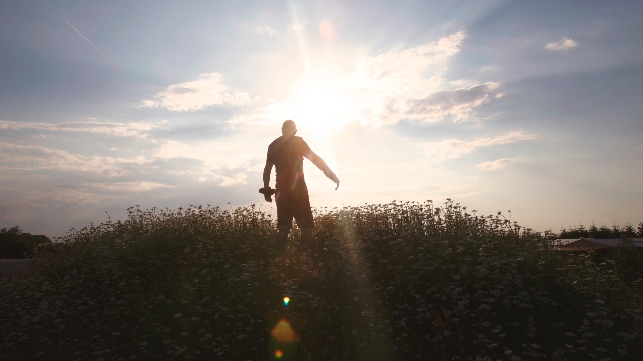Simple animation of a GIF beach ball We want to animate a raster image, derived from a photograph. To keep things simple and clear we are just going to move a photographic image (in GIF format) of a beach ball across a black background. Getting ready We need a suitable GIF image of an object that we want to animate. An example of one, named beachball.gif has been provided. How to do it... Copy a .gif fle from somewhere and paste it into a directory where you want to keep your work-in-progress pictures. Ensure that the path in our computer's fle system leads to the image to be used. In the example below, the instruction, ball = PhotoImage(file = "constr/pics2/beachball.gif") says that the image to be used will be found in a directory (folder) called pics2, which is a sub-folder of another folder called constr. Then execute the following code. # photoimage_animation_1.py #>>>>>>>>>>>>>>>>>>>>>>>> from Tkinter import * root = Tk() cycle_period = 100 cw = 300 # canvas width ch = 200 # canvas height canvas_1 = Canvas(root, width=cw, height=ch, bg="black") canvas_1.grid(row=0, column=1) posn_x = 10 posn_y = 10 shift_x = 2 shift_y = 1 ball = PhotoImage(file = "/constr/pics2/beachball.gif") for i in range(1,100): # end the program after 100 position shifts. posn_x += shift_x posn_y += shift_y canvas_1.create_image(posn_x,posn_y,anchor=NW, image=ball) canvas_1.update() # This refreshes the drawing on the canvas. canvas_1.after(cycle_period) # This makes execution pause for 100 milliseconds. canvas_1.delete(ALL) # This erases everything on the canvas. root.mainloop() How it Works The image of the beach ball is shifted across a canvas. The photo type images always occupy a rectangular area of screen. The size of this box, called the bounding box, is the size of the image. We have used a black background so the black corners on the image of our beach ball cannot be seen. The vector walking creature We make a pair of walking legs using the vector graphics. We want to use these legs together with pieces of raster images and see how far we can go in making appealing animations. We import Tkinter, math, and time modules. The math is needed to provide the trigonometry that sustains the geometric relations that move the parts of the leg in relation to each other. Getting ready We will be using Tkinter and time modules to animate the movement of lines and circles. You will see some trigonometry in the code. If you do not like mathematics you can just cut and paste the code without the need to understand exactly how the maths works. However, if you are a friend of mathematics it is fun to watch sine, cosine, and tangent working together to make a child smile. How to do it... Execute the program as shown in the previous image. # walking_creature_1.py # >>>>>>>>>>>>>>>> from Tkinter import * import math import time root = Tk() root.title("The thing that Strides") cw = 400 # canvas width ch = 100 # canvas height #GRAVITY = 4 chart_1 = Canvas(root, width=cw, height=ch, background="white") chart_1.grid(row=0, column=0) cycle_period = 100 # time between new positions of the ball (milliseconds). base_x = 20 base_y = 100 hip_h = 40 thy = 20 #=============================================== # Hip positions: Nhip = 2 x Nstep, the number of steps per foot per stride. hip_x = [0, 5, 10, 15, 20, 25, 30, 35, 40, 45, 50, 55, 60, 60, 60] #15 hip_y = [0, 8, 12, 16, 12, 8, 0, 0, 0, 8, 12, 16, 12, 8, 0] #15 step_x = [0, 10, 20, 30, 40, 50, 60, 60] # 8 = Nhip step_y = [0, 35, 45, 50, 43, 32, 10, 0] # The merging of the separate x and y lists into a single sequence. #================================== # Given a line joining two points xy0 and xy1, the base of an isosceles triangle, # as well as the length of one side, "thy" . This returns the coordinates of # the apex joining the equal-length sides. def kneePosition(x0, y0, x1, y1, thy): theta_1 = math.atan2((y1 - y0), (x1 - x0)) L1 = math.sqrt( (y1 - y0)**2 + (x1 - x0)**2) if L1/2 < thy: # The sign of alpha determines which way the knees bend. alpha = -math.acos(L1/(2*thy)) # Avian #alpha = math.acos(L1/(2*thy)) # Mammalian else: alpha = 0.0 theta_2 = alpha + theta_1 x_knee = x0 + thy * math.cos(theta_2) y_knee = y0 + thy * math.sin(theta_2) return x_knee, y_knee def animdelay(): chart_1.update() # This refreshes the drawing on the canvas. chart_1.after(cycle_period) # This makes execution pause for 200 milliseconds. chart_1.delete(ALL) # This erases *almost* everything on the canvas. # Does not delete the text from inside a function. bx_stay = base_x by_stay = base_y for j in range(0,11): # Number of steps to be taken - arbitrary. astep_x = 60*j bstep_x = astep_x + 30 cstep_x = 60*j + 15 aa = len(step_x) -1 for k in range(0,len(hip_x)-1): # Motion of the hips in a stride of each foot. cx0 = base_x + cstep_x + hip_x[k] cy0 = base_y - hip_h - hip_y[k] cx1 = base_x + cstep_x + hip_x[k+1] cy1 = base_y - hip_h - hip_y[k+1] chart_1.create_line(cx0, cy0 ,cx1 ,cy1) chart_1.create_oval(cx1-10 ,cy1-10 ,cx1+10 ,cy1+10, fill="orange") if k >= 0 and k <= len(step_x)-2: # Trajectory of the right foot. ax0 = base_x + astep_x + step_x[k] ax1 = base_x + astep_x + step_x[k+1] ay0 = base_y - step_y[k] ay1 = base_y - step_y[k+1] ax_stay = ax1 ay_stay = ay1 if k >= len(step_x)-1 and k <= 2*len(step_x)-2: # Trajectory of the left foot. bx0 = base_x + bstep_x + step_x[k-aa] bx1 = base_x + bstep_x + step_x[k-aa+1] by0 = base_y - step_y[k-aa] by1 = base_y - step_y[k-aa+1] bx_stay = bx1 by_stay = by1 aknee_xy = kneePosition(ax_stay, ay_stay, cx1, cy1, thy) chart_1.create_line(ax_stay, ay_stay ,aknee_xy[0], aknee_xy[1], width = 3, fill="orange") chart_1.create_line(cx1, cy1 ,aknee_xy[0], aknee_xy[1], width = 3, fill="orange") chart_1.create_oval(ax_stay-5 ,ay1-5 ,ax1+5 ,ay1+5, fill="green") chart_1.create_oval(bx_stay-5 ,by_stay-5 ,bx_stay+5 ,by_stay+5, fill="blue") bknee_xy = kneePosition(bx_stay, by_stay, cx1, cy1, thy) chart_1.create_line(bx_stay, by_stay ,bknee_xy[0], bknee_xy[1], width = 3, fill="pink") chart_1.create_line(cx1, cy1 ,bknee_xy[0], bknee_xy[1], width = 3, fill="pink") animdelay() root.mainloop() How it works... Without getting bogged down in detail, the strategy in the program consists of defning the motion of a foot while walking one stride. This motion is defned by eight relative positions given by the two lists step_x (horizontal) and step_y (vertical). The motion of the hips is given by a separate pair of x- and y-positions hip_x and hip_y. Trigonometry is used to work out the position of the knee on the assumption that the thigh and lower leg are the same length. The calculation is based on the sine rule taught in high school. Yes, we do learn useful things at school! The time-animation regulation instructions are assembled together as a function animdelay(). There's more In Python math module, two arc-tangent functions are available for calculating angles given the lengths of two adjacent sides. atan2(y,x) is the best because it takes care of the crazy things a tangent does on its way around a circle - tangent ficks from minus infnity to plus infnity as it passes through 90 degrees and any multiples thereof. A mathematical knee is quite happy to bend forward or backward in satisfying its equations. We make the sign of the angle negative for a backward-bending bird knee and positive for a forward bending mammalian knee. More Info Section 1 This animated walking hips-and-legs is used in the recipes that follow this to make a bird walk in the desert, a diplomat in palace grounds, and a spider in a forest. Bird with shoes walking in the Karroo We now coordinate the movement of four GIF images and the striding legs to make an Apteryx (a fightless bird like the kiwi) that walks. 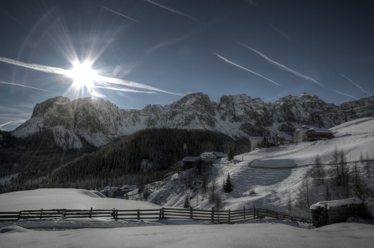Getting ready We need the following GIF images: A background picture of a suitable landscape A bird body without legs A pair of garish-colored shoes to make the viewer smile The walking avian legs of the previous recipe The images used are karroo.gif, apteryx1.gif, and shoe1.gif. Note that the images of the bird and the shoe have transparent backgrounds which means there is no rectangular background to be seen surrounding the bird or the shoe. In the recipe following this one, we will see the simplest way to achieve the necessary transparency. How to do it... Execute the program shown in the usual way. # walking_birdy_1.py # >>>>>>>>>>>>>>>> from Tkinter import * import math import time root = Tk() root.title("A Walking birdy gif and shoes images") cw = 800 # canvas width ch = 200 # canvas height #GRAVITY = 4 chart_1 = Canvas(root, width=cw, height=ch, background="white") chart_1.grid(row=0, column=0) cycle_period = 80 # time between new positions of the ball (milliseconds). im_backdrop = "/constr/pics1/karoo.gif" im_bird = "/constr/pics1/apteryx1.gif" im_shoe = "/constr/pics1/shoe1.gif" birdy =PhotoImage(file= im_bird) shoey =PhotoImage(file= im_shoe) backdrop = PhotoImage(file= im_backdrop) chart_1.create_image(0 ,0 ,anchor=NW, image=backdrop) base_x = 20 base_y = 190 hip_h = 70 thy = 60 #========================================== # Hip positions: Nhip = 2 x Nstep, the number of steps per foot per stride. hip_x = [0, 5, 10, 15, 20, 25, 30, 35, 40, 45, 50, 55, 60, 60, 60] #15 hip_y = [0, 8, 12, 16, 12, 8, 0, 0, 0, 8, 12, 16, 12, 8, 0] #15 step_x = [0, 10, 20, 30, 40, 50, 60, 60] # 8 = Nhip step_y = [0, 35, 45, 50, 43, 32, 10, 0] #============================================= # Given a line joining two points xy0 and xy1, the base of an isosceles triangle, # as well as the length of one side, "thy" this returns the coordinates of # the apex joining the equal-length sides. def kneePosition(x0, y0, x1, y1, thy): theta_1 = math.atan2(-(y1 - y0), (x1 - x0)) L1 = math.sqrt( (y1 - y0)**2 + (x1 - x0)**2) alpha = math.atan2(hip_h,L1) theta_2 = -(theta_1 - alpha) x_knee = x0 + thy * math.cos(theta_2) y_knee = y0 + thy * math.sin(theta_2) return x_knee, y_knee def animdelay(): chart_1.update() # Refresh the drawing on the canvas. chart_1.after(cycle_period) # Pause execution pause for X millise-conds. chart_1.delete("walking") # Erases everything on the canvas. bx_stay = base_x by_stay = base_y for j in range(0,13): # Number of steps to be taken - arbitrary. astep_x = 60*j bstep_x = astep_x + 30 cstep_x = 60*j + 15 aa = len(step_x) -1 for k in range(0,len(hip_x)-1): # Motion of the hips in a stride of each foot. cx0 = base_x + cstep_x + hip_x[k] cy0 = base_y - hip_h - hip_y[k] cx1 = base_x + cstep_x + hip_x[k+1] cy1 = base_y - hip_h - hip_y[k+1] #chart_1.create_image(cx1-55 ,cy1+20 ,anchor=SW, image=birdy, tag="walking") if k >= 0 and k <= len(step_x)-2: # Trajectory of the right foot. ax0 = base_x + astep_x + step_x[k] ax1 = base_x + astep_x + step_x[k+1] ay0 = base_y - 10 - step_y[k] ay1 = base_y - 10 -step_y[k+1] ax_stay = ax1 ay_stay = ay1 if k >= len(step_x)-1 and k <= 2*len(step_x)-2: # Trajectory of the left foot. bx0 = base_x + bstep_x + step_x[k-aa] bx1 = base_x + bstep_x + step_x[k-aa+1] by0 = base_y - 10 - step_y[k-aa] by1 = base_y - 10 - step_y[k-aa+1] bx_stay = bx1 by_stay = by1 chart_1.create_image(ax_stay-5 ,ay_stay + 10 ,anchor=SW, im-age=shoey, tag="walking") chart_1.create_image(bx_stay-5 ,by_stay + 10 ,anchor=SW, im-age=shoey, tag="walking") aknee_xy = kneePosition(ax_stay, ay_stay, cx1, cy1, thy) chart_1.create_line(ax_stay, ay_stay-15 ,aknee_xy[0], aknee_xy[1], width = 5, fill="orange", tag="walking") chart_1.create_line(cx1, cy1 ,aknee_xy[0], aknee_xy[1], width = 5, fill="orange", tag="walking") bknee_xy = kneePosition(bx_stay, by_stay, cx1, cy1, thy) chart_1.create_line(bx_stay, by_stay-15 ,bknee_xy[0], bknee_xy[1], width = 5, fill="pink", tag="walking") chart_1.create_line(cx1, cy1 ,bknee_xy[0], bknee_xy[1], width = 5, fill="pink", tag="walking") chart_1.create_image(cx1-55 ,cy1+20 ,anchor=SW, image=birdy, tag="walking") animdelay() root.mainloop() How it works... The same remarks concerning the trigonometry made in the previous recipe apply here. What we see here now is the ease with which vector objects and raster images can be combined once suitable GIF images have been prepared. There's more... For teachers and their students who want to make lessons on a computer, these techniques offer all kinds of possibilities like history tours and re-enactments, geography tours, and, science experiments. Get the students to do projects telling stories. Animated year books?

In this article, we'll cover how to use corpus readers and create custom corpora. At the same time, you'll learn how to use the existing corpus data that comes with NLTK. We'll also cover creating custom corpus readers, which can be used when your corpus is not in a file format that NLTK already recognizes, or if your corpus is not in files at all, but instead is located in a database such as MongoDB. Setting up a custom corpus A corpus is a collection of text documents, and corpora is the plural of corpus. So a custom corpus is really just a bunch of text files in a directory, often alongside many other directories of text files. Getting ready You should already have the NLTK data package installed, following the instructions at http://www.nltk.org/data. We'll assume that the data is installed to C:nltk_data on Windows, and /usr/share/nltk_data on Linux, Unix, or Mac OS X. How to do it... NLTK defines a list of data directories, or paths, in nltk.data.path. Our custom corpora must be within one of these paths so it can be found by NLTK. So as not to conflict with the official data package, we'll create a custom nltk_data directory in our home directory. Here's some Python code to create this directory and verify that it is in the list of known paths specified by nltk.data.path: >>> import os, os.path >>> path = os.path.expanduser('~/nltk_data') >>> if not os.path.exists(path): ... os.mkdir(path) >>> os.path.exists(path) True >>> import nltk.data >>> path in nltk.data.path True If the last line, path in nltk.data.path, is True, then you should now have a nltk_ data directory in your home directory. The path should be %UserProfile%nltk_data on Windows, or ~/nltk_data on Unix, Linux, or Mac OS X. For simplicity, I'll refer to the directory as ~/nltk_data. If the last line does not return True, try creating the nltk_data directory manually in your home directory, then verify that the absolute path is in nltk.data.path. It's essential to ensure that this directory exists and is in nltk.data.path before continuing. Once you have your nltk_data directory, the convention is that corpora reside in a corpora subdirectory. Create this corpora directory within the nltk_data directory, so that the path is ~/nltk_data/corpora. Finally, we'll create a subdirectory in corpora to hold our custom corpus. Let's call it cookbook, giving us the full path of ~/nltk_data/corpora/cookbook. Now we can create a simple word list file and make sure it loads. The source code for this article can be downloaded here. Consider a word list file called mywords.txt. Put this file into ~/nltk_data/corpora/cookbook/. Now we can use nltk.data.load() to load the file. >>> import nltk.data >>> nltk.data.load('corpora/cookbook/mywords.txt', format='raw') 'nltkn' We need to specify format='raw' since nltk.data.load() doesn't know how to interpret .txt files. As we'll see, it does know how to interpret a number of other file formats. How it works... The nltk.data.load() function recognizes a number of formats, such as 'raw', 'pickle', and 'yaml'. If no format is specified, then it tries to guess the format based on the file's extension. In the previous case, we have a .txt file, which is not a recognized extension, so we have to specify the 'raw' format. But if we used a file that ended in .yaml, then we would not need to specify the format. Filenames passed in to nltk.data.load() can be absolute or relative paths. Relative paths must be relative to one of the paths specified in nltk.data.path. The file is found using nltk.data.find(path), which searches all known paths combined with the relative path. Absolute paths do not require a search, and are used as is. There's more... For most corpora access, you won't actually need to use nltk.data.load, as that will be handled by the CorpusReader classes covered in the following recipes. But it's a good function to be familiar with for loading .pickle files and .yaml files, plus it introduces the idea of putting all of your data files into a path known by NLTK. Loading a YAML file If you put the synonyms.yaml file into ~/nltk_data/corpora/cookbook (next to mywords.txt), you can use nltk.data. load() to load it without specifying a format. >>> import nltk.data >>> nltk.data.load('corpora/cookbook/synonyms.yaml') {'bday': 'birthday'} This assumes that PyYAML is installed. If not, you can find download and installation instructions at http://pyyaml.org/wiki/PyYAML. See also In the next recipes, we'll cover various corpus readers, and then in the Lazy corpus loading recipe, we'll use the LazyCorpusLoader, which expects corpus data to be in a corpora subdirectory of one of the paths specified by nltk.data.path. Creating a word list corpus The WordListCorpusReader is one of the simplest CorpusReader classes. It provides access to a file containing a list of words, one word per line. Getting ready We need to start by creating a word list file. This could be a single column CSV file, or just a normal text file with one word per line. Let's create a file named wordlist that looks like this: nltk corpus corpora wordnet How to do it... Now we can instantiate a WordListCorpusReader that will produce a list of words from our file. It takes two arguments: the directory path containing the files, and a list of filenames. If you open the Python console in the same directory as the files, then '.' can be used as the directory path. Otherwise, you must use a directory path such as: 'nltk_data/corpora/ cookbook'. >>> from nltk.corpus.reader import WordListCorpusReader >>> reader = WordListCorpusReader('.', ['wordlist']) >>> reader.words() ['nltk', 'corpus', 'corpora', 'wordnet'] >>> reader.fileids() ['wordlist'] How it works... WordListCorpusReader inherits from CorpusReader, which is a common base class for all corpus readers. CorpusReader does all the work of identifying which files to read, while WordListCorpus reads the files and tokenizes each line to produce a list of words. Here's an inheritance diagram: When you call the words() function, it calls nltk.tokenize.line_tokenize() on the raw file data, which you can access using the raw() function. >>> reader.raw() 'nltkncorpusncorporanwordnetn' >>> from nltk.tokenize import line_tokenize >>> line_tokenize(reader.raw()) ['nltk', 'corpus', 'corpora', 'wordnet'] There's more... The stopwords corpus is a good example of a multi-file WordListCorpusReader. Names corpus Another word list corpus that comes with NLTK is the names corpus. It contains two files: female.txt and male.txt, each containing a list of a few thousand common first names organized by gender. >>> from nltk.corpus import names >>> names.fileids() ['female.txt', 'male.txt'] >>> len(names.words('female.txt')) 5001 >>> len(names.words('male.txt')) 2943 English words NLTK also comes with a large list of English words. There's one file with 850 basic words, and another list with over 200,000 known English words. >>> from nltk.corpus import words >>> words.fileids() ['en', 'en-basic'] >>> len(words.words('en-basic')) 850 >>> len(words.words('en')) 234936 Creating a part-of-speech tagged word corpus Part-of-speech tagging is the process of identifying the part-of-speech tag for a word. Most of the time, a tagger must first be trained on a training corpus. Let us take a look at how to create and use a training corpus of part-of-speech tagged words. Getting ready The simplest format for a tagged corpus is of the form "word/tag". Following is an excerpt from the brown corpus: The/at-tl expense/nn and/cc time/nn involved/vbn are/ber astronomical/ jj ./. Each word has a tag denoting its part-of-speech. For example, nn refers to a noun, while a tag that starts with vb is a verb. How to do it... If you were to put the previous excerpt into a file called brown.pos, you could then create a TaggedCorpusReader and do the following: >>> from nltk.corpus.reader import TaggedCorpusReader >>> reader = TaggedCorpusReader('.', r'.*.pos') >>> reader.words() ['The', 'expense', 'and', 'time', 'involved', 'are', ...] >>> reader.tagged_words() [('The', 'AT-TL'), ('expense', 'NN'), ('and', 'CC'), …] >>> reader.sents() [['The', 'expense', 'and', 'time', 'involved', 'are', 'astronomical', '.']] >>> reader.tagged_sents() [[('The', 'AT-TL'), ('expense', 'NN'), ('and', 'CC'), ('time', 'NN'), ('involved', 'VBN'), ('are', 'BER'), ('astronomical', 'JJ'), ('.', '.')]] >>> reader.paras() [[['The', 'expense', 'and', 'time', 'involved', 'are', 'astronomical', '.']]] >>> reader.tagged_paras() [[[('The', 'AT-TL'), ('expense', 'NN'), ('and', 'CC'), ('time', 'NN'), ('involved', 'VBN'), ('are', 'BER'), ('astronomical', 'JJ'), ('.', '.')]]] How it works... This time, instead of naming the file explicitly, we use a regular expression, r'.*.pos', to match all files whose name ends with .pos. We could have done the same thing as we did with the WordListCorpusReader, and pass ['brown.pos'] as the second argument, but this way you can see how to include multiple files in a corpus without naming each one explicitly. TaggedCorpusReader provides a number of methods for extracting text from a corpus. First, you can get a list of all words, or a list of tagged tokens. A tagged token is simply a tuple of (word, tag). Next, you can get a list of every sentence, and also every tagged sentence, where the sentence is itself a list of words or tagged tokens. Finally, you can get a list of paragraphs, where each paragraph is a list of sentences, and each sentence is a list of words or tagged tokens. Here's an inheritance diagram listing all the major methods: There's more... The functions demonstrated in the previous diagram all depend on tokenizers for splitting the text. TaggedCorpusReader tries to have good defaults, but you can customize them by passing in your own tokenizers at initialization time. Customizing the word tokenizer The default word tokenizer is an instance of nltk.tokenize.WhitespaceTokenizer. If you want to use a different tokenizer, you can pass that in as word_tokenizer. >>> from nltk.tokenize import SpaceTokenizer >>> reader = TaggedCorpusReader('.', r'.*.pos', word_ tokenizer=SpaceTokenizer()) >>> reader.words() ['The', 'expense', 'and', 'time', 'involved', 'are', ...] Customizing the sentence tokenizer The default sentence tokenizer is an instance of nltk.tokenize.RegexpTokenize with 'n' to identify the gaps. It assumes that each sentence is on a line all by itself, and individual sentences do not have line breaks. To customize this, you can pass in your own tokenizer as sent_tokenizer. >>> from nltk.tokenize import LineTokenizer >>> reader = TaggedCorpusReader('.', r'.*.pos', sent_ tokenizer=LineTokenizer()) >>> reader.sents() [['The', 'expense', 'and', 'time', 'involved', 'are', 'astronomical', '.']] Customizing the paragraph block reader Paragraphs are assumed to be split by blank lines. This is done with the default para_ block_reader, which is nltk.corpus.reader.util.read_blankline_block. There are a number of other block reader functions in nltk.corpus.reader.util, whose purpose is to read blocks of text from a stream. Their usage will be covered in more detail in the later recipe, Creating a custom corpus view, where we'll create a custom corpus reader. Customizing the tag separator If you don't want to use '/' as the word/tag separator, you can pass an alternative string to TaggedCorpusReader for sep. The default is sep='/', but if you want to split words and tags with '|', such as 'word|tag', then you should pass in sep='|'. Simplifying tags with a tag mapping function If you'd like to somehow transform the part-of-speech tags, you can pass in a tag_mapping_ function at initialization, then call one of the tagged_* functions with simplify_ tags=True. Here's an example where we lowercase each tag: >>> reader = TaggedCorpusReader('.', r'.*.pos', tag_mapping_ function=lambda t: t.lower()) >>> reader.tagged_words(simplify_tags=True) [('The', 'at-tl'), ('expense', 'nn'), ('and', 'cc'), …] Calling tagged_words() without simplify_tags=True would produce the same result as if you did not pass in a tag_mapping_function. There are also a number of tag simplification functions defined in nltk.tag.simplify. These can be useful for reducing the number of different part-of-speech tags. >>> from nltk.tag import simplify >>> reader = TaggedCorpusReader('.', r'.*.pos', tag_mapping_ function=simplify.simplify_brown_tag) >>> reader.tagged_words(simplify_tags=True) [('The', 'DET'), ('expense', 'N'), ('and', 'CNJ'), ...] >>> reader = TaggedCorpusReader('.', r'.*.pos', tag_mapping_ function=simplify.simplify_tag) >>> reader.tagged_words(simplify_tags=True) [('The', 'A'), ('expense', 'N'), ('and', 'C'), ...]

Storing a frequency distribution in Redis` Redis is a data structure server that is one of the more popular NoSQL databases. Among other things, it provides a network accessible database for storing dictionaries (also known as hash maps). Building a FreqDist interface to a Redis hash map will allow us to create a persistent FreqDist that is accessible to multiple local and remote processes at the same time. Most Redis operations are atomic, so it's even possible to have multiple processes write to the FreqDist concurrently. Getting ready For this and subsequent recipes, we need to install both Redis and redis-py. A quick start install guide for Redis is available at http://code.google.com/p/redis/wiki/ QuickStart. To use hash maps, you should install at least version 2.0.0 (the latest version as of this writing). The Redis Python driver redis-py can be installed using pip install redis or easy_ install redis. Ensure you install at least version 2.0.0 to use hash maps. The redispy homepage is at http://github.com/andymccurdy/redis-py/. Once both are installed and a redis-server process is running, you're ready to go. Let's assume redis-server is running on localhost on port 6379 (the default host and port). How to do it... The FreqDist class extends the built-in dict class, which makes a FreqDist an enhanced dictionary. The FreqDist class provides two additional key methods: inc() and N(). The inc() method takes a single sample argument for the key, along with an optional count keyword argument that defaults to 1, and increments the value at sample by count. N() returns the number of sample outcomes, which is the sum of all the values in the frequency distribution. We can create an API-compatible class on top of Redis by extending a RedisHashMap (that will be explained in the next section), then implementing the inc() and N() methods. Since the FreqDist only stores integers, we also override a few other methods to ensure values are always integers. This RedisHashFreqDist (defined in redisprob.py) uses the hincrby command for the inc() method to increment the sample value by count, and sums all the values in the hash map for the N() method. from rediscollections import RedisHashMap class RedisHashFreqDist(RedisHashMap): def inc(self, sample, count=1): self._r.hincrby(self._name, sample, count) def N(self): return int(sum(self.values())) def __getitem__(self, key): return int(RedisHashMap.__getitem__(self, key) or 0) def values(self): return [int(v) for v in RedisHashMap.values(self)] def items(self): return [(k, int(v)) for (k, v) in RedisHashMap.items(self)] We can use this class just like a FreqDist. To instantiate it, we must pass a Redis connection and the name of our hash map. The name should be a unique reference to this particular FreqDist so that it doesn't clash with any other keys in Redis. >>> from redis import Redis >>> from redisprob import RedisHashFreqDist >>> r = Redis() >>> rhfd = RedisHashFreqDist(r, 'test') >>> len(rhfd) 0 >>> rhfd.inc('foo') >>> rhfd['foo'] 1 >>> rhfd.items() >>> len(rhfd) 1 The name of the hash map and the sample keys will be encoded to replace whitespace and & characters with _. This is because the Redis protocol uses these characters for communication. It's best if the name and keys don't include whitespace to begin with. How it works... Most of the work is done in the RedisHashMap class, found in rediscollections.py, which extends collections.MutableMapping, then overrides all methods that require Redis-specific commands. Here's an outline of each method that uses a specific Redis command: __len__(): Uses the hlen command to get the number of elements in the hash map __contains__(): Uses the hexists command to check if an element exists in the hash map __getitem__(): Uses the hget command to get a value from the hash map __setitem__(): Uses the hset command to set a value in the hash map __delitem__(): Uses the hdel command to remove a value from the hash map keys(): Uses the hkeys command to get all the keys in the hash map values(): Uses the hvals command to get all the values in the hash map items(): Uses the hgetall command to get a dictionary containing all the keys and values in the hash map clear(): Uses the delete command to remove the entire hash map from Redis Extending collections.MutableMapping provides a number of other dict compatible methods based on the previous methods, such as update() and setdefault(), so we don't have to implement them ourselves. The initialization used for the RedisHashFreqDist is actually implemented here, and requires a Redis connection and a name for the hash map. The connection and name are both stored internally to use with all the subsequent commands. As mentioned before, whitespace is replaced by underscore in the name and all keys, for compatibility with the Redis network protocol. import collections, re white = r'[s&]+' def encode_key(key): return re.sub(white, '_', key.strip()) class RedisHashMap(collections.MutableMapping): def __init__(self, r, name): self._r = r self._name = encode_key(name) def __iter__(self): return iter(self.items()) def __len__(self): return self._r.hlen(self._name) def __contains__(self, key): return self._r.hexists(self._name, encode_key(key)) def __getitem__(self, key): return self._r.hget(self._name, encode_key(key)) def __setitem__(self, key, val): self._r.hset(self._name, encode_key(key), val) def __delitem__(self, key): self._r.hdel(self._name, encode_key(key)) def keys(self): return self._r.hkeys(self._name) def values(self): return self._r.hvals(self._name) def items(self): return self._r.hgetall(self._name).items() def get(self, key, default=0): return self[key] or default def iteritems(self): return iter(self) def clear(self): self._r.delete(self._name) There's more... The RedisHashMap can be used by itself as a persistent key-value dictionary. However, while the hash map can support a large number of keys and arbitrary string values, its storage structure is more optimal for integer values and smaller numbers of keys. However, don't let that stop you from taking full advantage of Redis. It's very fast (for a network server) and does its best to efficiently encode whatever data you throw at it. While Redis is quite fast for a network database, it will be significantly slower than the in-memory FreqDist. There's no way around this, but while you sacrifice speed, you gain persistence and the ability to do concurrent processing. See also In the next recipe, we'll create a conditional frequency distribution based on the Redis frequency distribution created here. Storing a conditional frequency distribution in Redis The nltk.probability.ConditionalFreqDist class is a container for FreqDist instances, with one FreqDist per condition. It is used to count frequencies that are dependent on another condition, such as another word or a class label. Here, we'll create an API-compatible class on top of Redis using the RedisHashFreqDist from the previous recipe. Getting ready As in the previous recipe, you'll need to have Redis and redis-py installed with an instance of redis-server running. How to do it... We define a RedisConditionalHashFreqDist class in redisprob.py that extends nltk.probability.ConditionalFreqDist and overrides the __contains__() and __getitem__() methods. We then override __getitem__() so we can create an instance of RedisHashFreqDist instead of a FreqDist, and override __contains__() so we can call encode_key() from the rediscollections module before checking if the RedisHashFreqDist exists. from nltk.probability import ConditionalFreqDist from rediscollections import encode_key class RedisConditionalHashFreqDist(ConditionalFreqDist): def __init__(self, r, name, cond_samples=None): self._r = r self._name = name ConditionalFreqDist.__init__(self, cond_samples) # initialize self._fdists for all matching keys for key in self._r.keys(encode_key('%s:*' % name)): condition = key.split(':')[1] self[condition] # calls self.__getitem__(condition) def __contains__(self, condition): return encode_key(condition) in self._fdists def __getitem__(self, condition): if condition not in self._fdists: key = '%s:%s' % (self._name, condition) self._fdists[condition] = RedisHashFreqDist(self._r, key) return self._fdists[condition] def clear(self): for fdist in self._fdists.values(): fdist.clear() An instance of this class can be created by passing in a Redis connection and a base name. After that, it works just like a ConditionalFreqDist. >>> from redis import Redis >>> from redisprob import RedisConditionalHashFreqDist >>> r = Redis() >>> rchfd = RedisConditionalHashFreqDist(r, 'condhash') >>> rchfd.N() 0 >>> rchfd.conditions() [] >>> rchfd['cond1'].inc('foo') >>> rchfd.N() 1 >>> rchfd['cond1']['foo'] 1 >>> rchfd.conditions() ['cond1'] >>> rchfd.clear() How it works... The RedisConditionalHashFreqDist uses name prefixes to reference RedisHashFreqDist instances. The name passed in to the RedisConditionalHashFreqDist is a base name that is combined with each condition to create a unique name for each RedisHashFreqDist. For example, if the base name of the RedisConditionalHashFreqDist is 'condhash', and the condition is 'cond1', then the final name for the RedisHashFreqDist is 'condhash:cond1'. This naming pattern is used at initialization to find all the existing hash maps using the keys command. By searching for all keys matching 'condhash:*', we can identify all the existing conditions and create an instance of RedisHashFreqDist for each. Combining strings with colons is a common naming convention for Redis keys as a way to define namespaces. In our case, each RedisConditionalHashFreqDist instance defines a single namespace of hash maps. The ConditionalFreqDist class stores an internal dictionary at self._fdists that is a mapping of condition to FreqDist. The RedisConditionalHashFreqDist class still uses self._fdists, but the values are instances of RedisHashFreqDist instead of FreqDist. self._fdists is created when we call ConditionalFreqDist.__init__(), and values are initialized as necessary in the __getitem__() method. There's more... RedisConditionalHashFreqDist also defines a clear() method. This is a helper method that calls clear() on all the internal RedisHashFreqDist instances. The clear() method is not defined in ConditionalFreqDist. See also The previous recipe covers the RedisHashFreqDist in detail.

  Python Text Processing with NLTK 2.0 Cookbook Use Python's NLTK suite of libraries to maximize your Natural Language Processing capabilities. Quickly get to grips with Natural Language Processing – with Text Analysis, Text Mining, and beyond Learn how machines and crawlers interpret and process natural languages Easily work with huge amounts of data and learn how to handle distributed processing Part of Packt's Cookbook series: Each recipe is a carefully organized sequence of instructions to complete the task as efficiently as possible     Introduction NLTK is great for in-memory single-processor natural language processing. However, there are times when you have a lot of data to process and want to take advantage of multiple CPUs, multi-core CPUs, and even multiple computers. Or perhaps you want to store frequencies and probabilities in a persistent, shared database so multiple processes can access it simultaneously. For the first case, we'll be using execnet to do parallel and distributed processing with NLTK. For the second case, you'll learn how to use the Redis data structure server/database to store frequency distributions and more. Distributed tagging with execnet Execnet is a distributed execution library for python. It allows you to create gateways and channels for remote code execution. A gateway is a connection from the calling process to a remote environment. The remote environment can be a local subprocess or an SSH connection to a remote node. A channel is created from a gateway and handles communication between the channel creator and the remote code. Since many NLTK processes require 100 percent CPU utilization during computation, execnet is an ideal way to distribute that computation for maximum resource usage. You can create one gateway per CPU core, and it doesn't matter whether the cores are in your local computer or spread across remote machines. In many situations, you only need to have the trained objects and data on a single machine, and can send the objects and data to the remote nodes as needed. Getting ready You'll need to install execnet for this to work. It should be as simple as sudo pip install execnet or sudo easy_install execnet. The current version of execnet, as of this writing, is 1.0.8. The execnet homepage, which has API documentation and examples, is at http://codespeak.net/execnet/. How to do it... We start by importing the required modules, as well as an additional module remote_tag. py that will be explained in the next section. We also need to import pickle so we can serialize the tagger. Execnet does not natively know how to deal with complex objects such as a part-of-speech tagger, so we must dump the tagger to a string using pickle.dumps(). We'll use the default tagger that's used by the nltk.tag.pos_tag() function, but you could load and dump any pre-trained part-of-speech tagger as long as it implements the TaggerI interface. Once we have a serialized tagger, we start execnet by making a gateway with execnet. makegateway(). The default gateway creates a Python subprocess, and we can call the remote_exec() method with the remote_tag module to create a channel. With an open channel, we send over the serialized tagger and then the first tokenized sentence of the treebank corpus. You don't have to do any special serialization of simple types such as lists and tuples, since execnet already knows how to handle serializing the built-in types. Now if we call channel.receive(), we get back a tagged sentence that is equivalent to the first tagged sentence in the treebank corpus, so we know the tagging worked. We end by exiting the gateway, which closes the channel and kills the subprocess. >>> import execnet, remote_tag, nltk.tag, nltk.data >>> from nltk.corpus import treebank >>> import cPickle as pickle >>> tagger = pickle.dumps(nltk.data.load(nltk.tag._POS_TAGGER)) >>> gw = execnet.makegateway() >>> channel = gw.remote_exec(remote_tag) >>> channel.send(tagger) >>> channel.send(treebank.sents()[0]) >>> tagged_sentence = channel.receive() >>> tagged_sentence == treebank.tagged_sents()[0] True >>> gw.exit() Visually, the communication process looks like this: How it works... The gateway's remote_exec() method takes a single argument that can be one of the following three types: A string of code to execute remotely. The name of a pure function that will be serialized and executed remotely. The name of a pure module whose source will be executed remotely. We use the third option with the remote_tag.py module, which is defined as follows: import cPickle as pickle if __name__ == '__channelexec__': tagger = pickle.loads(channel.receive()) for sentence in channel: channel.send(tagger.tag(sentence)) A pure module is a module that is self-contained. It can only access Python modules that are available where it executes, and does not have access to any variables or states that exist wherever the gateway is initially created. To detect that the module is being executed by execnet, you can look at the __name__ variable. If it's equal to '__channelexec__', then it is being used to create a remote channel. This is similar to doing if __name__ == '__ main__' to check if a module is being executed on the command line. The first thing we do is call channel.receive() to get the serialized tagger, which we load using pickle.loads(). You may notice that channel is not imported anywhere—that's because it is included in the global namespace of the module. Any module that execnet executes remotely has access to the channel variable in order to communicate with the channel` creator. Once we have the tagger, we iteratively tag() each tokenized sentence that we receive from the channel. This allows us to tag as many sentences as the sender wants to send, as iteration will not stop until the channel is closed. What we've essentially created is a compute node for part-of-speech tagging that dedicates 100 percent of its resources to tagging whatever sentences it receives. As long as the channel remains open, the node is available for processing. There's more... This is a simple example that opens a single gateway and channel. But execnet can do a lot more, such as opening multiple channels to increase parallel processing, as well as opening gateways to remote hosts over SSH to do distributed processing. Multiple channels We can create multiple channels, one per gateway, to make the processing more parallel. Each gateway creates a new subprocess (or remote interpreter if using an SSH gateway) and we use one channel per gateway for communication. Once we've created two channels, we can combine them using the MultiChannel class, which allows us to iterate over the channels, and make a receive queue to receive messages from each channel. After creating each channel and sending the tagger, we cycle through the channels to send an even number of sentences to each channel for tagging. Then we collect all the responses from the queue. A call to queue.get() will return a 2-tuple of (channel, message) in case you need to know which channel the message came from. If you don't want to wait forever, you can also pass a timeout keyword argument with the maximum number of seconds you want to wait, as in queue.get(timeout=4). This can be a good way to handle network errors. Once all the tagged sentences have been collected, we can exit the gateways. Here's the code: >>> import itertools >>> gw1 = execnet.makegateway() >>> gw2 = execnet.makegateway() >>> ch1 = gw1.remote_exec(remote_tag) >>> ch1.send(tagger) >>> ch2 = gw2.remote_exec(remote_tag) >>> ch2.send(tagger) >>> mch = execnet.MultiChannel([ch1, ch2]) >>> queue = mch.make_receive_queue() >>> channels = itertools.cycle(mch) >>> for sentence in treebank.sents()[:4]: ... channel = channels.next() ... channel.send(sentence) >>> tagged_sentences = [] >>> for i in range(4): ... channel, tagged_sentence = queue.get() ... tagged_sentences.append(tagged_sentence) >>> len(tagged_sentences) 4 >>> gw1.exit() >>> gw2.exit() Local versus remote gateways The default gateway spec is popen, which creates a Python subprocess on the local machine. This means execnet.makegateway() is equivalent to execnet. makegateway('popen'). If you have passwordless SSH access to a remote machine, then you can create a remote gateway using execnet.makegateway('ssh=remotehost') where remotehost should be the hostname of the machine. A SSH gateway spawns a new Python interpreter for executing the code remotely. As long as the code you're using for remote execution is pure, you only need a Python interpreter on the remote machine. Channels work exactly the same no matter what kind of gateway is used; the only difference will be communication time. This means you can mix and match local subprocesses with remote interpreters to distribute your computations across many machines in a network. There are many more details on gateways in the API documentation at http://codespeak.net/execnet/basics.html.

Statistical Analysis with R Take control of your data and produce superior statistical analysis with R. An easy introduction for people who are new to R, with plenty of strong examples for you to work through This book will take you on a journey to learn R as the strategist for an ancient Chinese kingdom! A step by step guide to understand R, its benefits, and how to use it to maximize the impact of your data analysis A practical guide to conduct and communicate your data analysis with R in the most effective manner           Read more about this book       (For more resources on R, see here.) Time for action — creating a line chart The ever popular line chart, or line graph, depicts relationships as continuous series of connected data points. Line charts are particularly useful for visualizing specific values and trends over time. Just as a line chart is an extension of a scatterplot in the non-digital realm, a line chart is created using an extended form of the plot(...) function in R. Let us explore how to extend the plot(...) function to create line charts in R: Use the type argument within the plot(...) function to create a line chart that depicts a single relationship between two variables: > #create a line chart that depicts the durations of past fire attacks> #get the data to be used in the chart> lineFireDurationDataX <- c(1:30)> lineFireDurationDataY <- subsetFire$DurationInDays> #customize the chart> lineFireDurationMain <- "Duration of Past Fire Attacks"> lineFireDurationLabX <- "Battle Number"> lineFireDurationLabY <- "Duration in Days"> #use the type argument to connect the data points with a line> lineFireDurationType <- "o"> #use plot(...) to create and display the line chart> plot(x = lineFireDurationDataX, y = lineFireDurationDataY,main = lineFireDurationMain, xlab = lineFireDurationLabX,ylab = lineFireDurationLabY, type = lineFireDurationType) Your chart will be displayed in the graphic window, as follows: What just happened? We expanded our use of the plot(...) function to generate a line chart and encountered a new data notation in the process. Let us review these features. type In the plot(...) function, the type argument determines what kind of line, if any, should be used to connect a chart's data points. The type argument receives one of several character values, all of which are listed as follows: p: only points are plotted; this is the default value when type is undefined l: only lines are drawn, without any points o: both lines and points are drawn, with the lines overlapping the points b: both lines and points are drawn, with the lines broken where they intersect with points c: only lines are drawn, but they are broken where points would occur s: only the lines are drawn in step formation; the initial step begins at zero S: (uppercase) only the lines are drawn in step formation; the final step tails off at the last point h: vertical lines are drawn to represent each point n: no points nor lines are drawn Our chart, which represented the duration of past fire attacks, featured a line that overlapped the plotted points. First, we defined our desired line type in an R variable: > lineFireDurationType <- "o" Then the type argument was placed within our plot(...) function to generate the line chart: > plot(lineFireDurationDataX, lineFireDurationDataY,main = lineFireDurationMain, xlab = lineFireDurationLabX,ylab = lineFireDurationLabY,type = lineFireDurationType) Number-colon-number notation You may have noticed that we specified a vector for the x-axis data in our plot(...) function. > lineFireDurationDataX <- c(1:30) This vector used number-colon-number notation. Essentially, this notation has the effect of enumerating a range of values that lie between the number that precedes the colon and the number that follows it. To do so, it adds one to the beginning value until it reaches a final value that is equal to or less than the number that comes after the colon. For example, the code > 14:21 would yield eight whole numbers, beginning with 14 and ending with 21, as follows: [1] 14 15 16 17 18 19 20 21 Furthermore, the code > 14.2:21 would yield seven values, beginning with 14.2 and ending with 20.2, as follows: [1] 14.2 15.2 16.2 17.2 18.2 19.2 20.2 Number-colon-number notation is a useful way to enumerate a series of values without having to type each one individually. It can be used in any circumstance where a series of values is acceptable input into an R function. Number-colon-number notation can also enumerate values from high to low. For instance, 21:14 would yield a list of values beginning with 21 and ending with 14. Since we do not have exact dates or other identifying information for our 30 past battles, we simply enumerated the numbers 1 through 30 on the x-axis. This had the effect of assigning a generic identification number to each of our past battles, which in turn allowed us to plot the duration of each battle on the y axis. Pop quiz Which of the following is the type argument capable of? Drawing a line to connect or replace the points on a scatterplot. Drawing vertical or step lines. Drawing no points or lines. All of the above. What would the following line of code yield in the R console? > 1:50 A sequence of 50 whole numbers, in order from 1 to 50. A sequence of 50 whole numbers, in order from 50 to 1. A sequence of 50 random numbers, in order from 1 to 50. A sequence of 50 random numbers, in order from 50 to 1. Time for action — creating a box plot A useful way to convey a collection of summary statistics in a dataset is through the use of a box plot. This type of graph depicts a dataset's minimum and maximum, as well as its lower, median, and upper quartiles in a single diagram. Let us look at how box plots are created in R: Use the boxplot(...) function to create a box plot. > #create a box plot that depicts the number of soldiers required to launch a fire attack> #get the data to be used in the plot> boxplotFireShuSoldiersData <- subsetFire$ShuSoldiers> #customize the plot> boxPlotFireShuSoldiersLabelMain <- "Number of Soldiers Required to Launch a Fire Attack"> boxPlotFireShuSoldiersLabelX <- "Fire Attack Method"> boxPlotFireShuSoldiersLabelY <- "Number of Soldiers"> #use boxplot(...) to create and display the box plot> boxplot(x = boxplotFireShuSoldiersData,main = boxPlotFireShuSoldiersLabelMain,xlab = boxPlotFireShuSoldiersLabelX,ylab = boxPlotFireShuSoldiersLabelY) Your plot will be displayed in the graphic window, as shown in the following: Use the boxplot(...) function to create a box plot that compares multiple datasets. > #create a box plot that compares the number of soldiers required across the battle methods> #get the data formula to be used in the plot> boxplotAllMethodsShuSoldiersData <- battleHistory$ShuSoldiers ~ battleHistory$Method> #customize the plot> boxPlotAllMethodsShuSoldiersLabelMain <- "Number of Soldiers Required by Battle Method"> boxPlotAllMethodsShuSoldiersLabelX <- "Battle Method"> boxPlotAllMethodsShuSoldiersLabelY <- "Number of Soldiers"> #use boxplot(...) to create and display the box plot> boxplot(formula = boxplotAllMethodsShuSoldiersData,main = boxPlotAllMethodsShuSoldiersLabelMain,xlab = boxPlotAllMethodsShuSoldiersLabelX,ylab = boxPlotAllMethodsShuSoldiersLabelY) Your plot will be displayed in the graphic window, as shown in the following: What just happened? We just created two box plots using R's boxplot(...) function, one with a single box and one with multiple boxes. boxplot(...) We started by generating a single box plot that was composed of a dataset, main title, and x and y labels. The basic format for a single box plot is as follows: boxplot(x = dataset) The x argument contains the data to be plotted. Technically, only x is required to create a box plot, although you will often include additional arguments. Our boxplot(...) function used the main, xlab, and ylab arguments to display text on the plot, as shown: > boxplot(x = boxplotFireShuSoldiersData,main = boxPlotFireShuSoldiersLabelMain,xlab = boxPlotFireShuSoldiersLabelX,ylab = boxPlotFireShuSoldiersLabelY) Next, we created a multiple box plot that compared the number of Shu soldiers deployed by each battle method. The main, xlab, and ylab arguments remained from our single box plot, however our multiple box plot used the formula argument instead of x. Here, a formula allows us to break a dataset down into separate groups, thus yielding multiple boxes. The basic format for a multiple box plot is as follows: boxplot(formula = dataset ~ group) In our case, we took our entire Shu soldier dataset (battleHistory$ShuSoldiers) and separated it by battle method (battleHistory$Method): > boxplotAllMethodsShuSoldiersData <- battleHistory$ShuSoldiers ~ battleHistory$Method Once incorporated into the boxplot(...) function, this formula resulted in a plot that contained four distinct boxes—ambush, fire, head to head, and surround: > boxplot(formula = boxplotAllMethodsShuSoldiersData,main = boxPlotAllMethodsShuSoldiersLabelMain,xlab = boxPlotAllMethodsShuSoldiersLabelX,ylab = boxPlotAllMethodsShuSoldiersLabelY) Pop quiz Which of the following best describes the result of the following code? > boxplot(x = a) A single box plot of the a dataset. A single box plot of the x dataset. A multiple box plot of the a dataset that is grouped by x. A multiple box plot of the x dataset that is grouped by a. Which of the following best describes the result of the following code? > boxplot(formula = a ~ b) A single box plot of the a dataset. A single box plot of the b dataset. A multiple box plot of the a dataset that is grouped by b. A multiple box plot of the b dataset that is grouped by a.

  Statistical Analysis with R Take control of your data and produce superior statistical analysis with R. An easy introduction for people who are new to R, with plenty of strong examples for you to work through This book will take you on a journey to learn R as the strategist for an ancient Chinese kingdom! A step by step guide to understand R, its benefits, and how to use it to maximize the impact of your data analysis A practical guide to conduct and communicate your data analysis with R in the most effective manner           Read more about this book       (For more resources on R, see here.) Retracing and refining a complete analysis For demonstration purposes, it will be assumed that a fire attack was chosen as the optimal battle strategy. Throughout this segment, we will retrace the steps that lead us to this decision. Meanwhile, we will make sure to organize and clarify our analyses so they can be easily communicated to others. Suppose we determined our fire attack will take place 225 miles away in Anding, which houses 10,000 Wei soldiers. We will deploy 2,500 soldiers for a period of 7 days and assume that they are able to successfully execute the plans. Let us return to the beginning to develop this strategy with R in a clear and concise manner. Time for action – first steps To begin our analysis, we must first launch R and set our working directory: Launch R. The R console will be displayed. Set your R working directory using the setwd(dir) function. The following code is a hypothetical example. Your working directory should be a relevant location on your own computer. > #set the R working directory using setwd(dir)> setwd("/Users/johnmquick/rBeginnersGuide/") Verify that your working directory has been set to the proper location using the getwd() command : > #verify the location of your working directory> getwd()[1] "/Users/johnmquick/rBeginnersGuide/" What just happened? We prepared R to begin our analysis by launching the soft ware and setting our working directory. At this point, you should be very comfortable completing these steps. Time for action – data setup Next, we need to import our battle data into R and isolate the portion pertaining to past fire attacks: Copy the battleHistory.csv file into your R working directory. This file contains data from 120 previous battles between the Shu and Wei forces. Read the contents of battleHistory.csv into an R variable named battleHistory using the read.table(...) command: > #read the contents of battleHistory.csv into an R variable> #battleHistory contains data from 120 previous battlesbetween the Shu and Wei forces> battleHistory <- read.table("battleHistory.csv", TRUE, ",") Create a subset using the subset(data, ...) function and save it to a new variable named subsetFire: > #use the subset(data, ...) function to create a subset ofthe battleHistory dataset that contains data only from battlesin which the fire attack strategy was employed> subsetFire <- subset(battleHistory, battleHistory$Method =="fire") Verify the contents of the new subset. Note that the console should return 30 rows, all of which contain fire in the Method column: > #display the fire attack data subset> subsetFire What just happened? We imported our dataset and then created a subset containing our fire attack data. However, we used a slightly different function, called read.table(...), to import our external data into R. read.table(...) U p to this point, we have always used the read.csv() function to import data into R. However, you should know that there are oft en many ways to accomplish the same objectives in R. For instance, read.table(...) is a generic data import function that can handle a variety of file types. While it accepts several arguments, the following three are required to properly import a CSV file, like the one containing our battle history data: file: t he name of the file to be imported, along with its extension, in quotes header: whether or not the file contains column headings; TRUE for yes, FALSE (default) for no sep: t he character used to separate values in the file, in quotes Using these arguments, we were able to import the data in our battleHistory.csv into R. Since our file contained headings, we used a value of TRUE for the header argument and because it is a comma-separated values file, we used "," for our sep argument: > battleHistory <- read.table("battleHistory.csv", TRUE, ",") This is just one example of how a different technique can be used to achieve a similar outcome in R. We will continue to explore new methods in our upcoming activities. Pop quiz Suppose you wanted to import the following dataset, named newData into R. Which of the following read.table(...) functions would be best to use? 4,55,96,12 read.table("newData", FALSE, ",") read.table("newData", TRUE, ",") read.table("newData.csv", FALSE, ",") read.table("newData.csv", TRUE, ",") Time for action – data exploration To begin our analysis, we will examine the summary statistics and correlations of our data. These will give us an overview of the data and inform our subsequent analyses: Generate a summary of the fire attack subset using summary(object): > #generate a summary of the fire subset> summaryFire <- summary(subsetFire)> #display the summary> summaryFire Before calculating correlations, we will have to convert our nonnumeric data from the Method, SuccessfullyExecuted, and Result columns into numeric form. Re code the Method column using as.numeric(data): > #represent categorical data numerically usingas.numeric(data)> #recode the Method column into Fire = 1> numericMethodFire <- as.numeric(subsetFire$Method) - 1 Recode the SuccessfullyExecuted column using as.numeric(data): > #recode the SuccessfullyExecuted column into N = 0 and Y = 1> numericExecutionFire <-as.numeric(subsetFire$SuccessfullyExecuted) - 1 Recode the Result column using as.numeric(data): > #recode the Result column into Defeat = 0 and Victory = 1> numericResultFire <- as.numeric(subsetFire$Result) - 1 With the Method, SuccessfullyExecuted, and Result columns coded into numeric form, let us now add them back into our fire dataset. Save the data in our recoded variables back into the original dataset: > #save the data in the numeric Method, SuccessfullyExecuted,and Result columns back into the fire attack dataset> subsetFire$Method <- numericMethodFire> subsetFire$SuccessfullyExecuted <- numericExecutionFire> subsetFire$Result <- numericResultFire Display the numeric version of the fire attack subset. Notice that all of the columns now contain numeric data; it will look like the following: Having replaced our original text values in the SuccessfullyExecuted and Result columns with numeric data, we can now calculate all of the correlations in the dataset using the cor(data) function: > #use cor(data) to calculate all of the correlations in thefire attack dataset> cor(subsetFire) Note that the error message and NA values in our correlation output result from the fact that our Method column contains only a single value. This is irrelevant to our analysis and can be ignored. What just happened? Initially, we calculated summary statistics for our fire attack dataset using the summary(object) function. From this information, we can derive the following useful insights about our past battles: The rating of the Shu army's performance in fire attacks has ranged from 10 to 100, with a mean of 45 Fire attack plans have been successfully executed 10 out of 30 times (33%) Fire attacks have resulted in victory 8 out of 30 times (27%) Successfully executed fire attacks have resulted in victory 8 out of 10 times (80%), while unsuccessful attacks have never resulted in victory The number of Shu soldiers engaged in fire attacks has ranged from 100 to 10,000 with a mean of 2,052 The number of Wei soldiers engaged in fire attacks has ranged from 1,500 to 50,000 with a mean of 12,333 The duration of fire attacks has ranged from 1 to 14 days with a mean of 7 Next, we recoded the text values in our dataset's Method, SuccessfullyExecuted, and Result columns into numeric form. Aft er adding the data from these variables back into our our original dataset, we were able to calculate all of its correlations. This allowed us to learn even more about our past battle data: The performance rating of a fire attack has been highly correlated with successful execution of the battle plans (0.92) and the battle's result (0.90), but not strongly correlated with the other variables. The execution of a fire attack has been moderately negatively correlated with the duration of the attack, such that a longer attack leads to a lesser chance of success (-0.46). The numbers of Shu and Wei soldiers engaged are highly correlated with each other (0.74), but not strongly correlated with the other variables. The insights gleaned from our summary statistics and correlations put us in a prime position to begin developing our regression model. Pop quiz Which of the following is a benefit of adding a text variable back into its original dataset aft er it has been recoded into numeric form? Calculation functions can be executed on the recoded variable. Calculation functions can be executed on the other variables in the dataset. Calculation functions can be executed on the entire dataset. There is no benefit.

Statistical Analysis with R Take control of your data and produce superior statistical analysis with R. An easy introduction for people who are new to R, with plenty of strong examples for you to work through This book will take you on a journey to learn R as the strategist for an ancient Chinese kingdom! A step by step guide to understand R, its benefits, and how to use it to maximize the impact of your data analysis A practical guide to conduct and communicate your data analysis with R in the most effective manner       Charts, graphs, and plots in R R features several options for creating charts, graphs, and plots. In this article, we will explore the generation and customization of these visuals, as well as methods for saving and exporting them for use outside of R. The following visuals will be covered in this article: Bar graphs Scatterplots Line charts Box plots Histograms Pie charts Time for action — creating a bar chart A bar chart or bar graph is a common visual that uses rectangles to depict the values of different items. Bar graphs are especially useful when comparing data over time or between diverse groups. Let us create a bar chart in R: Open R and set your working directory: > #set the R working directory > #replace the sample location with one that is relevant to you > setwd("/Users/johnmquick/rBeginnersGuide/") Use the barplot(...) function to create a bar chart: > #create a bar chart that compares the mean durations of the battle methods > #calculate the mean duration of each battle method > meanDurationFire <- mean(subsetFire$DurationInDays) > meanDurationAmbush <- mean(subsetAmbush$DurationInDays) > meanDurationHeadToHead <- mean(subsetHeadToHead$DurationInDays) > meanDurationSurround <- mean(subsetSurround$DurationInDays) > #use a vector to define the chart's bar values > barAllMethodsDurationBars <- c(meanDurationFire, meanDurationAmbush, meanDurationHeadToHead, meanDurationSurround) > #use barplot(...) to create and display the bar chart > barplot(height = barAllMethodsDurationBars) Your chart will be displayed in the graphic window, similar to the following: What just happened? You created your first graphic in R. Let us examine the barplot(...) function that we used to generate our bar chart, along with the new R components that we encountered. barplot(...) We created a bar chart that compared the mean durations of battles between the different combat methods. As it turns out, there is only one required argument in the barplot(...) function. This height argument receives a series of values that specify the length of each bar. Therefore, the barplot(...) function, at its simplest, takes on the following form: barplot(height = heightValues) Accordingly, our bar chart function reflected this same format: > barplot(height = barAllMethodsDurationBars) Vectors We stored the heights of our chart's bars in a vector variable. In R, a vector is a series of data. R's c(...) function can be used to create a vector from one or more data points. For example, the numbers 1, 2, 3, 4, and 5 can be arranged into a vector like so: > #arrange the numbers 1, 2, 3, 4, and 5 into a vector > numberVector <- c(1, 2, 3, 4, 5) Similarly, text data can also be placed into vector form, so long as the values are contained within quotation marks: > #arrange the letters a, b, c, d, and e into a vector > textVector <- c("a", "b", "c", "d", "e") Our vector defined the values for our bars: > #use a vector to define the chart's bar values > barAllMethodsDurationBars <- c(meanDurationFire, meanDurationAmbush, meanDurationHeadToHead, meanDurationSurround) Many function arguments in R require vector input. Hence, it is very common to use and encounter the c(...) function when working in R. Graphic window When you executed your barplot(...) function in the R console, the graphic window opened to display it. The graphic window will have different names across different operating systems, but its purpose and function remain the same. For example, in Mac OS X, the graphic window is named Quartz. For the remainder of this article, all R graphics will be displayed without the graphics window frame, which will allow us to focus on the visuals themselves. Pop quiz When entering text into a vector using the c(...) function, what characters must surround each text value? Quotation marks Parenthesis Asterisks Percent signs   What is the purpose of the R graphic window? To debug graphics functions To execute graphics functions To edit graphics To display graphics