Building a smart gardening system
In this section, we will develop a smart gardening system. We will use a PID controller to manage all inputs from our sensors, which will be used in decision system. We'll measure soil moisture, temperature, and humidity as parameters for our system. To keep it simple for now, we'll only use one parameter, soil moisture level.
A high-level architecture can be seen in the following figure:
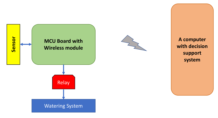
You can replace the MCU board and computer with a mini computer such as a Raspberry Pi. If you use a Raspberry Pi, you should remember that it does not have an analog input pin so you need an additional chip ADC, for instance the MCP3008, to work with analog input.
Assuming the watering system is connected via a relay, if we want to water the garden or farm, we just send digital value 1 to a relay. Some designs use a motor.
Let's build!
Introducing the PID controller
Proportional-integral-derivative (PID) control is the most common control algorithm used in the industry and has been universally accepted in industrial control. The basic idea behind a PID controller is to read a sensor and then compute the desired actuator output by calculating proportional, integral, and derivative responses and summing those three components to compute the output. The design of a general PID controller is as follows:
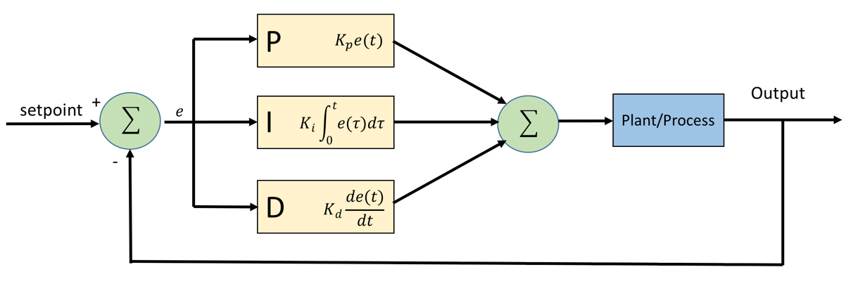
Furthermore, a PID controller formula can be defined as follows:
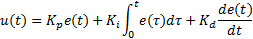

represents the coefficients for the proportional, integral, and derivative. These parameters are non-negative values. The variable

represents the tracking error, the difference between the desired input value i and the actual output y. This error signal

will be sent to the PID controller.
Implementing a PID controller in Python
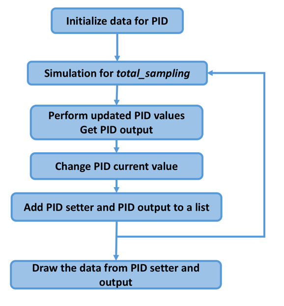
In this section, we'll build a Python application to implement a PID controller. In general, our program flowchart can be described as follows:
We should not build a PID library from scratch. You can translate the PID controller formula into Python code easily. For implementation, I'm using the PID class from https://github.com/ivmech/ivPID. The following the PID.py file:
import time
class PID:
"""PID Controller
"""
def __init__(self, P=0.2, I=0.0, D=0.0):
self.Kp = P
self.Ki = I
self.Kd = D
self.sample_time = 0.00
self.current_time = time.time()
self.last_time = self.current_time
self.clear()
def clear(self):
"""Clears PID computations and coefficients"""
self.SetPoint = 0.0
self.PTerm = 0.0
self.ITerm = 0.0
self.DTerm = 0.0
self.last_error = 0.0
# Windup Guard
self.int_error = 0.0
self.windup_guard = 20.0
self.output = 0.0
def update(self, feedback_value):
"""Calculates PID value for given reference feedback
.. math::
u(t) = K_p e(t) + K_i \int_{0}^{t} e(t)dt + K_d {de}/{dt}
.. figure:: images/pid_1.png
:align: center
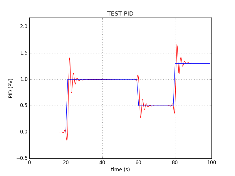
Test PID with Kp=1.2, Ki=1, Kd=0.001 (test_pid.py)
""
error = self.SetPoint - feedback_value
self.current_time = time.time()
delta_time = self.current_time - self.last_time
delta_error = error - self.last_error
if (delta_time >= self.sample_time):
self.PTerm = self.Kp * error
self.ITerm += error * delta_time
if (self.ITerm < -self.windup_guard):
self.ITerm = -self.windup_guard
elif (self.ITerm > self.windup_guard):
self.ITerm = self.windup_guard
self.DTerm = 0.0
if delta_time > 0:
self.DTerm = delta_error / delta_time
# Remember last time and last error for next calculation
self.last_time = self.current_time
self.last_error = error
self.output = self.PTerm + (self.Ki * self.ITerm) + (self.Kd * self.DTerm)
def setKp(self, proportional_gain):
"""Determines how aggressively the PID reacts to the current error with setting Proportional Gain"""
self.Kp = proportional_gain
def setKi(self, integral_gain):
"""Determines how aggressively the PID reacts to the current error with setting Integral Gain"""
self.Ki = integral_gain
def setKd(self, derivative_gain):
"""Determines how aggressively the PID reacts to the current error with setting Derivative Gain"""
self.Kd = derivative_gain
def setWindup(self, windup):
"""Integral windup, also known as integrator windup or reset windup,
refers to the situation in a PID feedback controller where
a large change in setpoint occurs (say a positive change)
and the integral terms accumulates a significant error during the rise (windup), thus overshooting and continuing
to increase as this accumulated error is unwound
(offset by errors in the other direction).
The specific problem is the excess overshooting.
"""
self.windup_guard = windup
def setSampleTime(self, sample_time):
"""PID that should be updated at a regular interval.
Based on a pre-determined sample time, the PID decides if it should compute or return immediately.
"""
self.sample_time = sample_time For testing, we'll create a simple program for simulation. We need libraries such as numpy, scipy, pandas, patsy, and matplotlib. Firstly, you should install python-dev for Python development. Type these commands on a Raspberry Pi terminal:
$ sudo apt-get update
$ sudo apt-get install python-dev
Now you can install the numpy, scipy, pandas, and patsy libraries. Open a Raspberry Pi terminal and type these commands:
$ sudo apt-get install python-scipy
$ pip install numpy scipy pandas patsy
The last step is to install the matplotlib library from the source code. Type these commands into the Raspberry Pi terminal:
$ git clone https://github.com/matplotlib/matplotlib
$ cd matplotlib
$ python setup.py build
$ sudo python setup.py install
After the required libraries are installed, we can test our PID.py code. Create a script with the following contents:
import matplotlib
matplotlib.use('Agg')

import PID
import time
import matplotlib.pyplot as plt
import numpy as np
from scipy.interpolate import spline


P = 1.4
I = 1
D = 0.001
pid = PID.PID(P, I, D)

pid.SetPoint = 0.0
pid.setSampleTime(0.01)

total_sampling = 100
feedback = 0

feedback_list = []
time_list = []
setpoint_list = []

print("simulating....")
for i in range(1, total_sampling):
    pid.update(feedback)
    output = pid.output
    if pid.SetPoint > 0:
        feedback += (output - (1 / i))

    if 20 < i < 60:
        pid.SetPoint = 1

    if 60 <= i < 80:
        pid.SetPoint = 0.5

    if i >= 80:
        pid.SetPoint = 1.3

    time.sleep(0.02)

    feedback_list.append(feedback)
    setpoint_list.append(pid.SetPoint)
    time_list.append(i)

time_sm = np.array(time_list)
time_smooth = np.linspace(time_sm.min(), time_sm.max(), 300)
feedback_smooth = spline(time_list, feedback_list, time_smooth)

fig1 = plt.gcf()
fig1.subplots_adjust(bottom=0.15)

plt.plot(time_smooth, feedback_smooth, color='red')
plt.plot(time_list, setpoint_list, color='blue')
plt.xlim((0, total_sampling))
plt.ylim((min(feedback_list) - 0.5, max(feedback_list) + 0.5))
plt.xlabel('time (s)')
plt.ylabel('PID (PV)')
plt.title('TEST PID')


plt.grid(True)
print("saving...")
fig1.savefig('result.png', dpi=100)
Save this program into a file called test_pid.py. Then run it:
$ python test_pid.pyThis program will generate result.png as a result of the PID process. A sample output is shown in the following screenshot. You can see that the blue line has the desired values and the red line is the output of the PID:
How it works
First, we define our PID parameters:
P = 1.4
I = 1
D = 0.001
pid = PID.PID(P, I, D)

pid.SetPoint = 0.0
pid.setSampleTime(0.01)

total_sampling = 100
feedback = 0

feedback_list = []
time_list = []
setpoint_list = []
After that, we compute the PID value during sampling. In this case, we set the desired output values as follows:
- Output 1 for sampling from 20 to 60
- Output 0.5 for sampling from 60 to 80
- Output 1.3 for sampling more than 80
for i in range(1, total_sampling):
    pid.update(feedback)
    output = pid.output
    if pid.SetPoint > 0:
        feedback += (output - (1 / i))

    if 20 < i < 60:
        pid.SetPoint = 1

    if 60 <= i < 80:
        pid.SetPoint = 0.5

    if i >= 80:
        pid.SetPoint = 1.3

    time.sleep(0.02)

    feedback_list.append(feedback)
    setpoint_list.append(pid.SetPoint)
    time_list.append(i)
The last step is to generate a report and save it into a file called result.png:
time_sm = np.array(time_list)
time_smooth = np.linspace(time_sm.min(), time_sm.max(), 300)
feedback_smooth = spline(time_list, feedback_list, time_smooth)

fig1 = plt.gcf()
fig1.subplots_adjust(bottom=0.15)

plt.plot(time_smooth, feedback_smooth, color='red')
plt.plot(time_list, setpoint_list, color='blue')
plt.xlim((0, total_sampling))
plt.ylim((min(feedback_list) - 0.5, max(feedback_list) + 0.5))
plt.xlabel('time (s)')
plt.ylabel('PID (PV)')
plt.title('TEST PID')


plt.grid(True)
print("saving...")
fig1.savefig('result.png', dpi=100)
Sending data from the Arduino to the server
Not all Arduino boards have the capability to communicate with a server. Some Arduino models have built-in Wi-Fi that can connect and send data to a server, for instance, the Arduino Yun, Arduino MKR1000, and Arduino UNO Wi-Fi.
You can use the HTTP or MQTT protocols to communicate with the server. After the server receives the data, it will perform a computation to determine its decision.
Controlling soil moisture using a PID controller
Now we can change our PID controller simulation using a real application. We use soil moisture to decide whether to pump water. The output of the measurement is used as feedback input for the PID controller.
If the PID output is a positive value, then we turn on the watering system. Otherwise, we stop it. This may not be a good approach but is a good way to show how PID controllers work. Soil moisture data is obtained from the Arduino through a wireless network.
Let's write this program:
import matplotlib
matplotlib.use('Agg')
import PID
import time
import matplotlib.pyplot as plt
import numpy as np
from scipy.interpolate import spline
P = 1.4
I = 1
D = 0.001
pid = PID.PID(P, I, D)
pid.SetPoint = 0.0
pid.setSampleTime(0.25) # a second
total_sampling = 100
sampling_i = 0
measurement = 0
feedback = 0
feedback_list = []
time_list = []
setpoint_list = []
def get_soil_moisture():
# reading from Arduino
# value 0 - 1023
return 200
print('PID controller is running..')
try:
while 1:
pid.update(feedback)
output = pid.output
soil_moisture = get_soil_moisture()
if soil_moisture is not None:
# # ## testing
# if 23 < sampling_i < 50:
# soil_moisture = 300
# if 65 <= sampling_i < 75:
# soil_moisture = 350
# if sampling_i >= 85:
# soil_moisture = 250
# # ################
if pid.SetPoint > 0:
feedback += soil_moisture + output
print('i={0} desired.soil_moisture={1:0.1f} soil_moisture={2:0.1f} pid.out={3:0.1f} feedback={4:0.1f}'
.format(sampling_i, pid.SetPoint, soil_moisture, output, feedback))
if output > 0:
print('turn on watering system')
elif output < 0:
print('turn off watering system')
if 20 < sampling_i < 60:
pid.SetPoint = 300 # soil_moisture
if 60 <= sampling_i < 80:
pid.SetPoint = 200 # soil_moisture
if sampling_i >= 80:
pid.SetPoint = 260 # soil_moisture
time.sleep(0.5)
sampling_i += 1
feedback_list.append(feedback)
setpoint_list.append(pid.SetPoint)
time_list.append(sampling_i)
if sampling_i >= total_sampling:
break
except KeyboardInterrupt:
print("exit")
print("pid controller done.")
print("generating a report...")
time_sm = np.array(time_list)
time_smooth = np.linspace(time_sm.min(), time_sm.max(), 300)
feedback_smooth = spline(time_list, feedback_list, time_smooth)
fig1 = plt.gcf()
fig1.subplots_adjust(bottom=0.15, left=0.1)
plt.plot(time_smooth, feedback_smooth, color='red')
plt.plot(time_list, setpoint_list, color='blue')
plt.xlim((0, total_sampling))
plt.ylim((min(feedback_list) - 0.5, max(feedback_list) + 0.5))
plt.xlabel('time (s)')
plt.ylabel('PID (PV)')
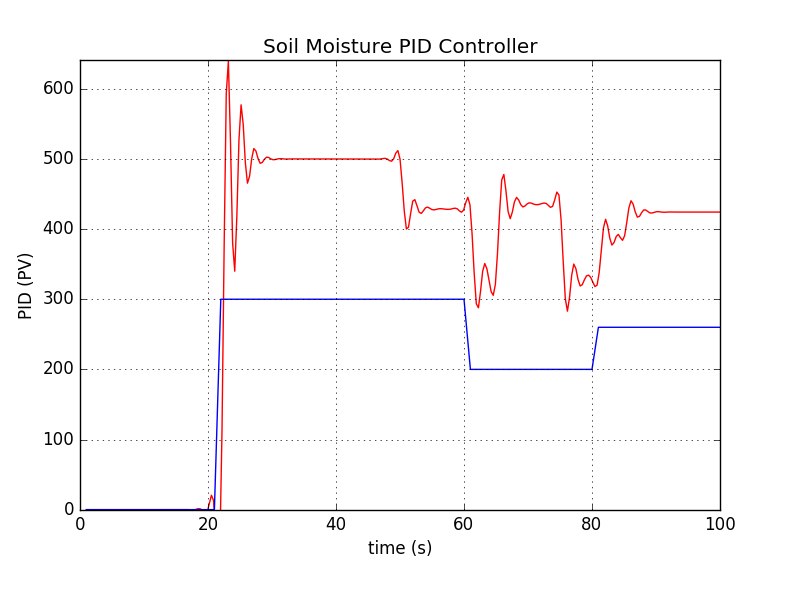
plt.title('Soil Moisture PID Controller')
plt.grid(True)
fig1.savefig('pid_soil_moisture.png', dpi=100)
print("finish") Save this program to a file called ch01_pid.py and run it like this:
$ sudo python ch01_pid.pyAfter executing the program, you should obtain a file called pid_soil_moisture.png. A sample output can be seen in the following figure:
How it works
Generally speaking, this program combines two things: reading the current soil moisture value through a soil moisture sensor and implementing a PID controller. After measuring the soil moisture level, we send the value to the PID controller program. The output of the PID controller will cause a certain action. In this case, it will turn on the watering machine.