Search icon CANCEL
Subscription
0
Cart icon
Your Cart (0 item)
Close icon
You have no products in your basket yet
Save more on your purchases! discount-offer-chevron-icon
Savings automatically calculated. No voucher code required.
Arrow left icon
All Products
Best Sellers
New Releases
Books
Videos
Audiobooks
Learning Hub
Newsletter Hub
Free Learning
Arrow right icon
timer SALE ENDS IN
0 Days
:
00 Hours
:
00 Minutes
:
00 Seconds
Arrow up icon
GO TO TOP
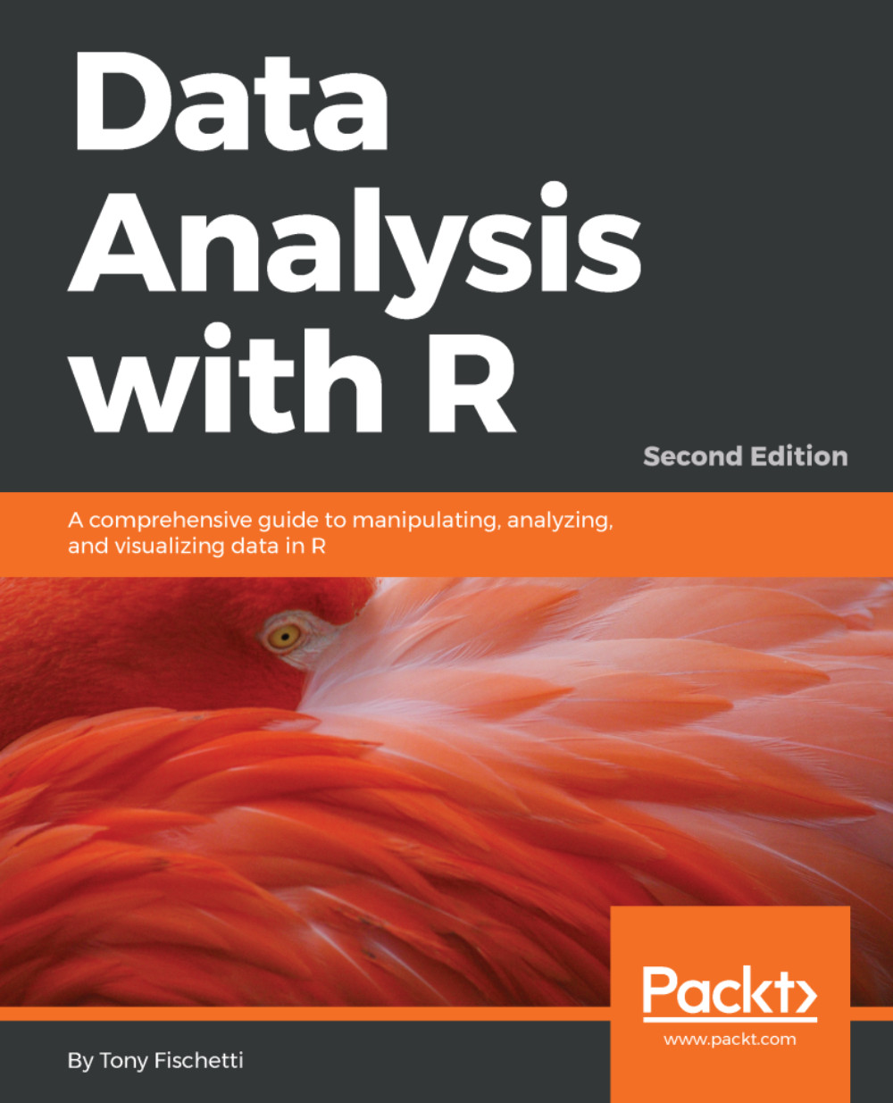
Data Analysis with R, Second Edition

You're reading from   Data Analysis with R, Second Edition A comprehensive guide to manipulating, analyzing, and visualizing data in R

Arrow left icon
Product type Paperback
Published in Mar 2018
Publisher Packt
ISBN-13 9781788393720
Length 570 pages
Edition 2nd Edition
Languages
Tools
Arrow right icon
Toc

Table of Contents (24) Chapters Close

Title Page
Copyright and Credits
Packt Upsell
Contributors
Preface
1. RefresheR FREE CHAPTER 2. The Shape of Data 3. Describing Relationships 4. Probability 5. Using Data To Reason About The World 6. Testing Hypotheses 7. Bayesian Methods 8. The Bootstrap 9. Predicting Continuous Variables 10. Predicting Categorical Variables 11. Predicting Changes with Time 12. Sources of Data 13. Dealing with Missing Data 14. Dealing with Messy Data 15. Dealing with Large Data 16. Working with Popular R Packages 17. Reproducibility and Best Practices 1. Other Books You May Enjoy Index

Be smart about your code


In many cases, the performance of the R code can be greatly improved by simple restructuring of the code; this doesn't change the output of the program, just the way it is represented. Restructurings of this type are often referred to as code refactoring. The refactorings that really make a difference performance-wise usually have to do with either improved allocation of memory or vectorization.

Allocation of memory

Refer all the way back to Chapter 5, Using Data to Reason About the World. Remember when we created a mock population of women's heights in the US, and we repeatedly took 10,000 samples of 40 from it to demonstrate the sampling distribution of the sample means? In a code comment, I mentioned in passing that the snippet numeric(10000) created an empty vector of 10,000 elements, but I never explained why we did that. Why didn't we just create a vector of 1, and continually tack on each new sample mean to the end of it? This is demonstrated as follows:

set...
lock icon The rest of the chapter is locked
Register for a free Packt account to unlock a world of extra content!
A free Packt account unlocks extra newsletters, articles, discounted offers, and much more. Start advancing your knowledge today.
Unlock this book and the full library FREE for 7 days
Get unlimited access to 7000+ expert-authored eBooks and videos courses covering every tech area you can think of
Renews at $15.99/month. Cancel anytime
Visually different images