In this article by Amarpreet Singh Bassan and Debarchan Sarkar, authors of Mastering SQL Server 2014 Data Mining, we will begin our discussion with an introduction to the data mining life cycle, and this article will focus on its first three stages. You are expected to have basic understanding of the Microsoft business intelligence stack and familiarity of terms such as extract, transform, and load (ETL), data warehouse, and so on.
(For more resources related to this topic, see here.)
Data mining life cycle
Before going into further details, it is important to understand the various stages of the data mining life cycle. The data mining life cycle can be broadly classified into the following steps:
- Understanding the business requirement.
- Understanding the data.
- Preparing the data for the analysis.
- Preparing the data mining models.
- Evaluating the results of the analysis prepared with the models.
- Deploying the models to the SQL Server Analysis Services Server.
- Repeating steps 1 to 6 in case the business requirement changes.
Let's look at each of these stages in detail.
The first and foremost task that needs to be well defined even before beginning the mining process is to identify the goals. This is a crucial part of the data mining exercise and you need to understand the following questions:
- What and whom are we targeting?
- What is the outcome we are targeting?
- What is the time frame for which we have the data and what is the target time period that our data is going to forecast?
- What would the success measures look like?
Let's define a classic problem and understand more about the preceding questions. We can use them to discuss how to extract the information rather than spending our time on defining the schema.
Consider an instance where you are a salesman for the AdventureWorks Cycle company, and you need to make predictions that could be used in marketing the products. The problem sounds simple and straightforward, but any serious data miner would immediately come up with many questions. Why? The answer lies in the exactness of the information being searched for. Let's discuss this in detail.
The problem statement comprises the words predictions and marketing. When we talk about predictions, there are several insights that we seek, namely:
- What is it that we are predicting? (for example: customers, product sales, and so on)
- What is the time period of the data that we are selecting for prediction?
- What time period are we going to have the prediction for?
- What is the expected outcome of the prediction exercise?
From the marketing point of view, several follow-up questions that must be answered are as follows:
- What is our target for marketing, a new product or an older product?
- Is our marketing strategy product centric or customer centric? Are we going to market our product irrespective of the customer classification, or are we marketing our product according to customer classification?
- On what timeline in the past is our marketing going to be based on?
We might observe that there are many questions that overlap the two categories and therefore, there is an opportunity to consolidate the questions and classify them as follows:
- What is the population that we are targeting?
- What are the factors that we will actually be looking at?
- What is the time period of the past data that we will be looking at?
- What is the time period in the future that we will be considering the data mining results for?
Let's throw some light on these aspects based on the AdventureWorks example. We will get answers to the preceding questions and arrive at a more refined problem statement.
What is the population that we are targeting? The target population might be classified according to the following aspects:
- Age
- Salary
- Number of kids
What are the factors that we are actually looking at? They might be classified as follows:
- Geographical location: The people living in hilly areas would prefer All Terrain Bikes (ATB) and the population on plains would prefer daily commute bikes.
- Household: The people living in posh areas would look for bikes with the latest gears and also look for accessories that are state of the art, whereas people in the suburban areas would mostly look for budgetary bikes.
- Affinity of components: The people who tend to buy bikes would also buy some accessories.
What is the time period of the past data that we would be looking at? Usually, the data that we get is quite huge and often consists of the information that we might very adequately label as noise. In order to sieve effective information, we will have to determine exactly how much into the past we should look; for example, we can look at the data for the past year, past two years, or past five years.
We also need to decide the future data that we will consider the data mining results for. We might be looking at predicting our market strategy for an upcoming festive season or throughout the year. We need to be aware that market trends change and so does people's needs and requirements. So we need to keep a time frame to refresh our findings to an optimal; for example, the predictions from the past 5 years data can be valid for the upcoming 2 or 3 years depending upon the results that we get.
Now that we have taken a closer look into the problem, let's redefine the problem more accurately. AdventureWorks has several stores in various locations and based on the location, we would like to get an insight on the following:
- Which products should be stocked where?
- Which products should be stocked together?
- How much of the products should be stocked?
- What is the trend of sales for a new product in an area?
It is not necessary that we will get answers to all the detailed questions but even if we keep looking for the answers to these questions, there would be several insights that we will get, which will help us make better business decisions.
Staging data
In this phase, we collect data from all the sources and dump them into a common repository, which can be any database system such as SQL Server, Oracle, and so on. Usually, an organization might have various applications to keep track of the data from various departments, and it is quite possible that all these applications might use a different database system to store the data. Thus, the staging phase is characterized by dumping the data from all the other data storage systems to a centralized repository.
Extract, transform, and load
This term is most common when we talk about data warehouse. As it is clear, ETL has the following three parts:
- Extract: The data is extracted from a different source database and other databases that might contain the information that we seek
- Transform: Some transformation is applied to the data to fit the operational needs, such as cleaning, calculation, removing duplicates, reformatting, and so on
- Load: The transformed data is loaded into the destination data store database
We usually believe that the ETL is only required till we load the data onto the data warehouse but this is not true. ETL can be used anywhere that we feel the need to do some transformation of data as shown in the following figure:

Data warehouse
As evident from the preceding figure, the next stage is the data warehouse. The AdventureWorksDW database is the outcome of the ETL applied to the staging database, which is AdventureWorks. We will now discuss the concepts of data warehousing and some best practices and then relate to these concepts with the help of AdventureWorksDW database.
Measures and dimensions
There are a few common terminologies you will encounter as you enter the world of data warehousing. They are as follows:
- Measure: Any business entity that can be aggregated or whose values can be ascertained in a numerical value is termed as measure, for example, sales, number of products, and so on
- Dimension: This is any business entity that lends some meaning to the measures, for example, in an organization, the quantity of goods sold is a measure but the month is a dimension
Schema
A schema, basically, determines the relationship of the various entities with each other. There are essentially two types of schema, namely:
- Star schema: This is a relationship where the measures have a direct relationship with the dimensions. Let's look at an instance wherein a seller has several stores that sell several products. The relationship of the tables based on the star schema will be as shown in the following screenshot:

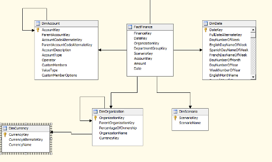
- Snowflake schema: This is a relationship wherein the measures may have a direct and indirect relationship with the dimensions. We will be designing a snowflake schema if we want a more detailed drill down of the data. Snowflake schema usually would involve hierarchies, as shown in the following screenshot:
Data mart
While a data warehouse is a more organization-wide repository of data, extracting data from such a huge repository might well be an uphill task. We segregate the data according to the department or the specialty that the data belongs to, so that we have much smaller sections of the data to work with and extract information from. We call these smaller data warehouses data marts.
Let's consider the sales for AdventureWorks cycles. To make any predictions on the sales of AdventureWorks, we will have to group all the tables associated with the sales together in a data mart. Based on the AdventureWorks database, we have the following table in the AdventureWorks sales data mart.
The Internet sales facts table has the following data:
[ProductKey]
[OrderDateKey]
[DueDateKey]
[ShipDateKey]
[CustomerKey]
[PromotionKey]
[CurrencyKey]
[SalesTerritoryKey]
[SalesOrderNumber]
[SalesOrderLineNumber]
[RevisionNumber]
[OrderQuantity]
[UnitPrice]
[ExtendedAmount]
[UnitPriceDiscountPct]
[DiscountAmount]
[ProductStandardCost]
[TotalProductCost]
[SalesAmount]
[TaxAmt]
[Freight]
[CarrierTrackingNumber]
[CustomerPONumber]
[OrderDate]
[DueDate]
[ShipDate]
From the preceding column, we can easily identify that if we need to separate the tables to perform the sales analysis alone, we can safely include the following:
- Product: This provides the following data:
[ProductKey]
[ListPrice]
- Date: This provides the following data:
[DateKey]
- Customer: This provides the following data:
[CustomerKey]
- Currency: This provides the following data:
[CurrencyKey]
- Sales territory: This provides the following data:
[SalesTerritoryKey]
The preceding data will provide the relevant dimensions and the facts that are already contained in the FactInternetSales table and hence, we can easily perform all the analysis pertaining to the sales of the organization.
Refreshing data
Based on the nature of the business and the requirements of the analysis, refreshing of data can be done either in parts wherein new or incremental data is added to the tables, or we can refresh the entire data wherein the tables are cleaned and filled with new data, which consists of the old and new data.
Let's discuss the preceding points in the context of the AdventureWorks database. We will take the employee table to begin with. The following is the list of columns in the employee table:
[BusinessEntityID]
,[NationalIDNumber]
,[LoginID]
,[OrganizationNode]
,[OrganizationLevel]
,[JobTitle]
,[BirthDate]
,[MaritalStatus]
,[Gender]
,[HireDate]
,[SalariedFlag]
,[VacationHours]
,[SickLeaveHours]
,[CurrentFlag]
,[rowguid]
,[ModifiedDate]
Considering an organization in the real world, we do not have a large number of employees leaving and joining the organization. So, it will not really make sense to have a procedure in place to reload the dimensions, prior to SQL 2008. When it comes to managing the changes in the dimensions table, Slowly Changing Dimensions (SCD) is worth a mention. We will briefly look at the SCD here. There are three types of SCD, namely:
- Type 1: The older values are overwritten by new values
- Type 2: A new row specifying the present value for the dimension is inserted
- Type 3: The column specifying TimeStamp from which the new value is effective is updated
Let's take the example of HireDate as a method of keeping track of the incremental loading. We will also have to maintain a small table that will keep a track of the data that is loaded from the employee table. So, we create a table as follows:
Create table employee_load_status(
HireDate DateTime,
LoadStatus varchar
);
The following script will load the employee table from the AdventureWorks database to the DimEmployee table in the AdventureWorksDW database:
With employee_loaded_date(HireDate) as
(select ISNULL(Max(HireDate),to_date('01-01-1900','MM-DD-YYYY')) from
employee_load_status where LoadStatus='success'
Union All
Select ISNULL(min(HireDate),to_date('01-01-1900','MM-DD-YYYY')) from
employee_load_status where LoadStatus='failed'
)
Insert into DimEmployee select * from employee where HireDate
>=(select Min(HireDate) from employee_loaded_date);
This will reload all the data from the date of the first failure till the present day.
A similar procedure can be followed to load the fact table but there is a catch. If we look at the sales table in the AdventureWorks table, we see the following columns:
[BusinessEntityID]
,[TerritoryID]
,[SalesQuota]
,[Bonus]
,[CommissionPct]
,[SalesYTD]
,[SalesLastYear]
,[rowguid]
,[ModifiedDate]
The SalesYTD column might change with every passing day, so do we perform a full load every day or do we perform an incremental load based on date? This will depend upon the procedure used to load the data in the sales table and the ModifiedDate column.
Assuming the ModifiedDate column reflects the date on which the load was performed, we also see that there is no table in the AdventureWorksDW that will use the SalesYTD field directly. We will have to apply some transformation to get the values of OrderQuantity, DateOfShipment, and so on.
Let's look at this with a simpler example. Consider we have the following sales table:
|
Name
Unlock access to the largest independent learning library in Tech for FREE!
Get unlimited access to 7500+ expert-authored eBooks and video courses covering every tech area you can think of.
Renews at €14.99/month. Cancel anytime
|
SalesAmount
|
Date
|
|
Rama
|
1000
|
11-02-2014
|
|
Shyama
|
2000
|
11-02-2014
|
Consider we have the following fact table:
We will have to think of whether to apply incremental load or a complete reload of the table based on our end needs. So the entries for the incremental load will look like this:
|
id
|
SalesAmount
|
Datekey
|
|
ra
|
1000
|
11-02-2014
|
|
Sh
|
2000
|
11-02-2014
|
|
Ra
|
4000
|
12-02-2014
|
|
Sh
|
5000
|
13-02-2014
|
Also, a complete reload will appear as shown here:
|
id
|
TotalSalesAmount
|
Datekey
|
|
Ra
|
5000
|
12-02-2014
|
|
Sh
|
7000
|
13-02-2014
|
Notice how the SalesAmount column changes to TotalSalesAmount depending on the load criteria.
Summary
In this article, we've covered the first three steps of any data mining process. We've considered the reasons why we would want to undertake a data mining activity and identified the goal we have in mind. We then looked to stage the data and cleanse it.
Resources for Article:
Further resources on this subject:

 United States
 Great Britain
 India
India
 Germany
 France
 Canada
 Russia
 Spain
Spain
 Brazil
 Australia
 South Africa
 Thailand
 Ukraine
 Switzerland
 Slovakia
 Luxembourg
 Hungary
 Romania
 Denmark
 Ireland
 Estonia
 Belgium
 Italy
Italy
 Finland
 Cyprus
 Lithuania
 Latvia
 Malta
Malta
 Netherlands
 Portugal
 Slovenia
 Sweden
 Argentina
 Colombia
 Ecuador
 Indonesia
 Mexico
 New Zealand
 Norway
 South Korea
 Taiwan
 Turkey
 Czechia
 Austria
 Greece
 Isle of Man
 Bulgaria
 Japan
Japan
 Philippines
 Poland
 Singapore
 Egypt
Egypt
 Chile
Chile
 Malaysia


