In this article by Paul Gerrard and Radia M. Johnson, the authors of Mastering Scientific Computation with R, we'll discuss the fundamental ideas underlying structural equation modeling, which are often overlooked in other books discussing structural equation modeling (SEM) in R, and then delve into how SEM is done in R. We will then discuss two R packages, OpenMx and lavaan. We can directly apply our discussion of the linear algebra underlying SEM using OpenMx. Because of this, we will go over OpenMx first. We will then discuss lavaan, which is probably more user friendly because it sweeps the matrices and linear algebra representations under the rug so that they are invisible unless the user really goes looking for them. Both packages continue to be developed and there will always be some features better supported in one of these packages than in the other.

(For more resources related to this topic, see here.)

SEM model fitting and estimation methods

To ultimately find a good solution, software has to use trial and error to come up with an implied covariance matrix that matches the observed covariance matrix as well as possible. The question is what does "as well as possible" mean? The answer to this is that the software must try to minimize some particular criterion, usually some sort of discrepancy function. Just what that criterion is depends on the estimation method used. The most commonly used estimation methods in SEM include:

Ordinary least squares (OLS) also called unweighted least squares
Generalized least squares (GLS)
Maximum likelihood (ML)

There are a number of other estimation methods as well, some of which can be done in R, but here we will stick with describing the most common ones. In general, OLS is the simplest and computationally cheapest estimation method. GLS is computationally more demanding, and ML is computationally more intensive. We will see why this is, as we discuss the details of these estimation methods.

Any SEM estimation method seeks to estimate model parameters that recreate the observed covariance matrix as well as possible. To evaluate how closely an implied covariance matrix matches an observed covariance matrix, we need a discrepancy function. If we assume multivariate normality of the observed variables, the following function can be used to assess discrepancy:

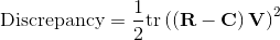
In the preceding figure, R is the observed covariance matrix, C is the implied covariance matrix, and V is a weight matrix.

The tr function refers to the trace function, which sums the elements of the main diagonal.

The choice of V varies based on the SEM estimation method:

For OLS, V = I
For GLS, V = R^-1

In the case of an ML estimation, we seek to minimize one of a number of similar criteria to describe ML, as follows:

In the preceding figure, n is the number of variables.

There are a couple of points worth noting here. GLS estimation inverts the observed correlation matrix, something computationally demanding with large matrices, but something that must only be done once. Alternatively, ML requires inversion of the implied covariance matrix, which changes with each iteration. Thus, each iteration requires the computationally demanding step of matrix inversion. With modern fast computers, this difference may not be noticeable, but with large SEM models, this might start to be quite time-consuming.

Assessing SEM model fit

The final question in an SEM model is how well the model explains the data. This is answered with the use of SEM measures of fit. Most of these measures are based on a chi-squared distribution. The fit criteria for GLS and ML (as well as a number of other estimation procedures such as asymptotic distribution-free methods) multiplied by N-1 is approximately chi-square distributed. Here, the capital N represents the number of observations in the dataset, as opposed to lower case n, which gives the number of variables. We compute degrees of freedom as the difference between the number of estimated parameters and the number of known covariances (that is, the total number of values in one triangle of an observed covariance matrix).

This gives way to the first test statistic for SEM models, a chi-squared significance level comparing our chi-square value to some minimum chi-square threshold to achieve statistical significance.

As with conventional chi-square testing, a chi-square value that is higher than some minimal threshold will reject the null hypothesis. Most experimental science features such as rejection supports the hypothesis of the experiment. This is not the case in SEM, where the null hypothesis is that the model fits the data. Thus, a non-significant chi-square is an indicator of model fit, whereas a significant chi-square rejects model fit. A notable limitation of this is that a greater sample size, greater N, will increase the chi-square value and will therefore increase the power to reject model fit. Thus, using conventional chi-squared testing will tend to support models developed in small samples and reject models developed in large samples.

The choice an interpretation of fit measures is a contentious one in SEM literature. However, as can be seen, chi-square has limitations. As such, other model fit criteria were developed that do not penalize models that fit in large samples (some may penalize models fit to small samples though). There are over a dozen indices, but the most common fit indices and interpretation information are as follows:

Comparative fit index: In this index, a higher value is better. Conventionally, a value of greater than 0.9 was considered an indicator of good model fit, but some might argue that a value of at least 0.95 is needed. This is relatively sample size insensitive.
Root mean square error of approximation: A value of under 0.08 (smaller is better) is often considered necessary to achieve model fit. However, this fit measure is quite sample size sensitive, penalizing small sample studies.
Tucker-Lewis index (Non-normed fit index): This is interpreted in a similar manner as the comparative fit index. Also, this is not very sample size sensitive.
Standardized root mean square residual: In this index, a lower value is better. A value of 0.06 or less is considered needed for model fit. Also, this may penalize small samples.

In the next section, we will show you how to actually fit SEM models in R and how to evaluate fit using fit measures.

Using OpenMx and matrix specification of an SEM

We went through the basic principles of SEM and discussed the basic computational approach by which this can be achieved. SEM remains an active area of research (with an entire journal devoted to it, Structural Equation Modeling), so there are many additional peculiarities, but rather than delving into all of them, we will start by delving into actually fitting an SEM model in R.

OpenMx is not in the CRAN repository, but it is easily obtainable from the OpenMx website, by typing the following in R:

source('http://openmx.psyc.virginia.edu/getOpenMx.R')"

Summarizing the OpenMx approach

In this example, we will use OpenMx by specifying matrices as mentioned earlier. To fit an OpenMx model, we need to first specify the model and then tell the software to attempt to fit the model. Model specification involves four components:

Specifying the model matrices; this has two parts:
- Declare starting values for the estimation
- Declaring which values can be estimated and which are fixed
Telling OpenMx the algebraic relationship of the matrices that should produce an implied covariance matrix
Giving an instruction for the model fitting criterion
Providing a source of data

The R commands that correspond to each of these steps are:

mxMatrix
mxAlgebra
mxMLObjective
mxData

We will then pass the objects created with each of these commands to create an SEM model using mxModel.

Explaining an entire example

First, to make things simple, we will store the FALSE and TRUE logical values in single letter variables, which will be convenient when we have matrices full of TRUE and FALSE values as follows:

F <- FALSE
T <- TRUE

Specifying the model matrices

Specifying matrices is done with the mxMatrix function, which returns an MxMatrix object. (Note that the object starts with a capital "M" while the function starts with a lowercase "m.") Specifying an MxMatrix is much like specifying a regular R matrix, but MxMatrices has some additional components. The most notable difference is that there are actually two different matrices used to create an MxMatrix. The first is a matrix of starting values, and the second is a matrix that tells which starting values are free to be estimated and which are not. If a starting value is not freely estimable, then it is a fixed constant. Since the actual starting values that we choose do not really matter too much in this case, we will just pick one as a starting value for all parameters that we would like to be estimated. Let's take a look at the following example:

mx.A <- mxMatrix(
type = "Full",
nrow=14,
ncol=14,
#Provide the Starting Values
values = c(
   0, 0, 0, 0, 0, 0, 0, 0, 0, 0, 0, 0, 1, 0,
   0, 0, 0, 0, 0, 0, 0, 0, 0, 0, 0, 0, 1, 0,
   0, 0, 0, 0, 0, 0, 0, 0, 0, 0, 0, 0, 1, 0,
   0, 0, 0, 0, 0, 0, 0, 0, 0, 0, 0, 0, 1, 0,
   0, 0, 0, 0, 0, 0, 0, 0, 0, 0, 0, 0, 0, 1,
   0, 0, 0, 0, 0, 0, 0, 0, 0, 0, 0, 0, 0, 1,
   0, 0, 0, 0, 0, 0, 0, 0, 0, 0, 0, 0, 0, 1,
   0, 0, 0, 0, 0, 0, 0, 0, 0, 0, 0, 0, 0, 1,
   0, 0, 0, 0, 0, 0, 0, 0, 0, 0, 0, 1, 0, 0,
   0, 0, 0, 0, 0, 0, 0, 0, 0, 0, 0, 1, 0, 0,
   0, 0, 0, 0, 0, 0, 0, 0, 0, 0, 0, 1, 0, 0,
   0, 0, 0, 0, 0, 0, 0, 0, 0, 0, 0, 0, 0, 0,
   0, 0, 0, 0, 0, 0, 0, 0, 0, 0, 0, 1, 0, 0,
   0, 0, 0, 0, 0, 0, 0, 0, 0, 0, 0, 1, 1, 0
),
#Tell R which values are free to be estimated   
free = c(
   F, F, F, F, F, F, F, F, F, F, F, F, F, F,
   F, F, F, F, F, F, F, F, F, F, F, F, T, F,
   F, F, F, F, F, F, F, F, F, F, F, F, T, F,
   F, F, F, F, F, F, F, F, F, F, F, F, T, F,
   F, F, F, F, F, F, F, F, F, F, F, F, F, F,
   F, F, F, F, F, F, F, F, F, F, F, F, F, T,
   F, F, F, F, F, F, F, F, F, F, F, F, F, T,
   F, F, F, F, F, F, F, F, F, F, F, F, F, T,
   F, F, F, F, F, F, F, F, F, F, F, F, F, F,
   F, F, F, F, F, F, F, F, F, F, F, T, F, F,
   F, F, F, F, F, F, F, F, F, F, F, T, F, F,
   F, F, F, F, F, F, F, F, F, F, F, F, F, F,
   F, F, F, F, F, F, F, F, F, F, F, T, F, F,
   F, F, F, F, F, F, F, F, F, F, F, T, T, F
),
byrow=TRUE,
 
#Provide a matrix name that will be used in model fitting
name="A",
)

We will now apply this same technique to the S matrix. Here, we will create two S matrices, S1 and S2. They differ simply in the starting values that they supply. We will later try to fit an SEM model using one matrix, and then the other to address problems with the first one. The difference is that S1 uses starting variances of 1 in the diagonal, and S2 uses starting variances of 5. Here, we will use the "symm" matrix type, which is a symmetric matrix. We could use the "full" matrix type, but by using "symm", we are saved from typing all of the symmetric values in the upper half of the matrix. Let's take a look at the following matrix:

mx.S1 <- mxMatrix("Symm", nrow=14, ncol=14,
values = c(
   1,
   0, 1,
   0, 0, 1,
   0, 1, 0, 1,
   1, 0, 0, 0, 1,
   0, 1, 0, 0, 0, 1,
   0, 0, 1, 0, 0, 0, 1,
   0, 0, 0, 1, 0, 1, 0, 1,
   0, 0, 0, 0, 0, 0, 0, 0, 1,
   0, 0, 0, 0, 0, 0, 0, 0, 0, 1,
   0, 0, 0, 0, 0, 0, 0, 0, 0, 0, 1,
   0, 0, 0, 0, 0, 0, 0, 0, 0, 0, 0, 1,
   0, 0, 0, 0, 0, 0, 0, 0, 0, 0, 0, 0, 1,
   0, 0, 0, 0, 0, 0, 0, 0, 0, 0, 0, 0, 0, 1
),
    
free = c(
   T,
   F, T,
   F, F, T,
   F, T, F, T,
   T, F, F, F, T,
   F, T, F, F, F, T,
   F, F, T, F, F, F, T,
   F, F, F, T, F, T, F, T,
   F, F, F, F, F, F, F, F, T,
   F, F, F, F, F, F, F, F, F, T,
   F, F, F, F, F, F, F, F, F, F, T,
   F, F, F, F, F, F, F, F, F, F, F, T,
   F, F, F, F, F, F, F, F, F, F, F, F, T,
   F, F, F, F, F, F, F, F, F, F, F, F, F, T
),
byrow=TRUE,
name="S"
)
 
#The alternative, S2 matrix:
mx.S2 <- mxMatrix("Symm", nrow=14, ncol=14,
values = c(
   5,
   0, 5,
   0, 0, 5,
   0, 1, 0, 5,
   1, 0, 0, 0, 5,
   0, 1, 0, 0, 0, 5,
   0, 0, 1, 0, 0, 0, 5,
   0, 0, 0, 1, 0, 1, 0, 5,
   0, 0, 0, 0, 0, 0, 0, 0, 5,
   0, 0, 0, 0, 0, 0, 0, 0, 0, 5,
   0, 0, 0, 0, 0, 0, 0, 0, 0, 0, 5,
   0, 0, 0, 0, 0, 0, 0, 0, 0, 0, 0, 5,
   0, 0, 0, 0, 0, 0, 0, 0, 0, 0, 0, 0, 5,
   0, 0, 0, 0, 0, 0, 0, 0, 0, 0, 0, 0, 0, 5
),
    
   free = c(
   T,
   F, T,
   F, F, T,
   F, T, F, T,
   T, F, F, F, T,
   F, T, F, F, F, T,
   F, F, T, F, F, F, T,
   F, F, F, T, F, T, F, T,
   F, F, F, F, F, F, F, F, T,
   F, F, F, F, F, F, F, F, F, T,
   F, F, F, F, F, F, F, F, F, F, T,
   F, F, F, F, F, F, F, F, F, F, F, T,
   F, F, F, F, F, F, F, F, F, F, F, F, T,
   F, F, F, F, F, F, F, F, F, F, F, F, F, T
),
byrow=TRUE,
name="S"
)
mx.Filter <- mxMatrix("Full", nrow=11, ncol=14,
values= c(
       1, 0, 0, 0, 0, 0, 0, 0, 0, 0, 0, 0, 0, 0,
     0, 1, 0, 0, 0, 0, 0, 0, 0, 0, 0, 0, 0, 0,
       0, 0, 1, 0, 0, 0, 0, 0, 0, 0, 0, 0, 0, 0,
       0, 0, 0, 1, 0, 0, 0, 0, 0, 0, 0, 0, 0, 0,
       0, 0, 0, 0, 1, 0, 0, 0, 0, 0, 0, 0, 0, 0,
       0, 0, 0, 0, 0, 1, 0, 0, 0, 0, 0, 0, 0, 0,
       0, 0, 0, 0, 0, 0, 1, 0, 0, 0, 0, 0, 0, 0,
       0, 0, 0, 0, 0, 0, 0, 1, 0, 0, 0, 0, 0, 0,
       0, 0, 0, 0, 0, 0, 0, 0, 1, 0, 0, 0, 0, 0,
       0, 0, 0, 0, 0, 0, 0, 0, 0, 1, 0, 0, 0, 0,
       0, 0, 0, 0, 0, 0, 0, 0, 0, 0, 1, 0, 0, 0
   ),
   free=FALSE,
   name="Filter",
   byrow = TRUE
)

And finally, we will create our identity and filter matrices the same way, as follows:

mx.I <- mxMatrix("Full", nrow=14, ncol=14,
   values= c(
       1, 0, 0, 0, 0, 0, 0, 0, 0, 0, 0, 0, 0, 0,
       0, 1, 0, 0, 0, 0, 0, 0, 0, 0, 0, 0, 0, 0,
       0, 0, 1, 0, 0, 0, 0, 0, 0, 0, 0, 0, 0, 0,
       0, 0, 0, 1, 0, 0, 0, 0, 0, 0, 0, 0, 0, 0,
       0, 0, 0, 0, 1, 0, 0, 0, 0, 0, 0, 0, 0, 0,
       0, 0, 0, 0, 0, 1, 0, 0, 0, 0, 0, 0, 0, 0,
       0, 0, 0, 0, 0, 0, 1, 0, 0, 0, 0, 0, 0, 0,
       0, 0, 0, 0, 0, 0, 0, 1, 0, 0, 0, 0, 0, 0,
       0, 0, 0, 0, 0, 0, 0, 0, 1, 0, 0, 0, 0, 0,
       0, 0, 0, 0, 0, 0, 0, 0, 0, 1, 0, 0, 0, 0,
       0, 0, 0, 0, 0, 0, 0, 0, 0, 0, 1, 0, 0, 0,
       0, 0, 0, 0, 0, 0, 0, 0, 0, 0, 0, 1, 0, 0,
       0, 0, 0, 0, 0, 0, 0, 0, 0, 0, 0, 0, 1, 0,
       0, 0, 0, 0, 0, 0, 0, 0, 0, 0, 0, 0, 0, 1
   ),
   free=FALSE,
   byrow = TRUE,
   name="I"
)

Fitting the model

Now, it is time to declare the model that we would like to fit using the mxModel command. This part includes steps 2 through step 4 mentioned earlier. Here, we will tell mxModel which matrices to use. We will then use the mxAlgegra command to tell R how the matrices should be combined to reproduce the implied covariance matrix. We will tell R to use ML estimation with the mxMLObjective command, and we will tell it to apply the estimation to a particular matrix algebra, which we named "C". This is simply the right-hand side of the McArdle McDonald equation. Finally, we will tell R where to get the data to use in model fitting using the following code:

factorModel.1 <- mxModel("Political Democracy Model",
#Model Matrices
mx.A,
mx.S1,
mx.Filter,
mx.I,
#Model Fitting Instructions
mxAlgebra(Filter %*% solve(I-A) %*% S %*% t(solve(I - A)) %*% t(Filter), name="C"),
     mxMLObjective("C", dimnames = names(PoliticalDemocracy)),
  
#Data to fit
mxData(cov(PoliticalDemocracy), type="cov", numObs=75)
)

Now, let's tell R to fit the model and summarize the results using mxRun, as follows:

summary(mxRun(factorModel.1))
Running Political Democracy Model
Error in summary(mxRun(factorModel.1)) :
error in evaluating the argument 'object' in selecting a method for function 'summary': Error: The job for model 'Political Democracy Model' exited abnormally with the error message: Expected covariance matrix is non-positive-definite.

Uh oh! We got an error message telling us that the expected covariance matrix is not positive definite. Our observed covariance matrix is positive definite but the implied covariance matrix (at least at first) is not. This is an effect of the fact that if we multiply our starting value matrices together as specified by the McArdle McDonald equation, we get a starting implied covariance matrix. If we perform an eigenvalue decomposition of this starting implied covariance matrix, then we will find that the last eigenvalue is negative. This means a negative variance does not make much sense, and this is what "not positive definite" refers to. The good news is that this is simply our starting values, so we can fix this if we modify our starting values. In this case, we can choose values of five along the diagonal of the S matrix, and get a positive definite starting implied covariance matrix. We can rerun this using the mx.S2 matrix specified earlier and the software will proceed as follows:

#Rerun with a positive definite matrix
 
factorModel.2 <- mxModel("Political Democracy Model",
#Model Matrices
mx.A,
mx.S2,
mx.Filter,
mx.I,
#Model Fitting Instructions
mxAlgebra(Filter %*% solve(I-A) %*% S %*% t(solve(I - A)) %*% t(Filter), name="C"),
   mxMLObjective("C", dimnames = names(PoliticalDemocracy)),
  
#Data to fit
mxData(cov(PoliticalDemocracy), type="cov", numObs=75)
)
 
summary(mxRun(factorModel.2))

This should provide a solution. As can be seen from the previous code, the parameters solved in the model are returned as matrix components. Just like we had to figure out how to go from paths to matrices, we now have to figure out how to go from matrices to paths (the reverse problem). In the following screenshot, we show just the first few free parameters:

structural-equation-modeling-and-confirmatory-factor-analysis-img-2

The preceding screenshot tells us that the parameter estimated in the position of the tenth row and twelfth column in the matrix A is 2.18. This corresponds to a path from the twelfth variable in the A matrix ind60, to the 10th variable in the matrix x2. Thus, the path coefficient from ind60 to x2 is 2.18.

There are a few other pieces of information here. The first one tells us that the model has not converged but is "Mx status Green." This means that the model was still converging when it stopped running (that is, it did not converge), but an optimal solution was still found and therefore, the results are likely reliable. Model fit information is also provided suggesting a pretty good model fit with CFI of 0.99 and RMSEA of 0.032.

This was a fair amount of work, and creating model matrices by hand from path diagrams can be quite tedious. For this reason, SEM fitting programs have generally adopted the ability to fit SEM by declaring paths rather than model matrices. OpenMx has the ability to allow declaration by paths, but applying model matrices has a few advantages. Principally, we get under the hood of SEM fitting. If we step back, we can see that OpenMx actually did very little for us that is specific to SEM. We told OpenMx how we wanted matrices multiplied together and which parameters of the matrix were free to be estimated. Instead of using the RAM specification, we could have passed the matrices of the LISREL or Bentler-Weeks models with the corresponding algebra methods to recreate an implied covariance matrix. This means that if we are trying to come up with our matrix specification, reproduce prior research, or apply a new SEM matrix specification method published in the literature, OpenMx gives us the power to do it. Also, for educators wishing to teach the underlying mathematical ideas of SEM, OpenMx is a very powerful tool.

Fitting SEM models using lavaan

If we were to describe OpenMx as the SEM equivalent of having a well-stocked pantry and full kitchen to create whatever you want, and you have the time and know how to do it, we might regard lavaan as a large freezer full of prepackaged microwavable dinners. It does not allow quite as much flexibility as OpenMx because it sweeps much of the work that we did by hand in OpenMx under the rug. Lavaan does use an internal matrix representation, but the user never has to see it. It is this sweeping under the rug that makes lavaan generally much easier to use. It is worth adding that the list of prepackaged features that are built into lavaan with minimal additional programming challenge many commercial SEM packages.

The lavaan syntax

The key to describing lavaan models is the model syntax, as follows:

X =~ Y: Y is a manifestation of the latent variable X
Y ~ X: Y is regressed on X
Y ~~ X: The covariance between Y and X can be estimated
Y ~ 1: This estimates the intercept for Y (implicitly requires mean structure)
Y | a*t1 + b*t2: Y has two thresholds that is a and b
Y ~ a * X: Y is regressed on X with coefficient a
Y ~ start(a) * X: Y is regressed on X; the starting value used for estimation is a

It may not be evident at first, but this model description language actually makes lavaan quite powerful. Wherever you have seen a or b in the previous examples, a variable or constant can be used in their place. The beauty of this is that multiple parameters can be constrained to be equal simply by assigning a single parameter name to them.

Using lavaan, we can fit a factor analysis model to our physical functioning dataset with only a few lines of code:

phys.func.data <- read.csv('phys_func.csv')[-1]
names(phys.func.data) <- LETTERS[1:20]

R has a built-in vector named LETTERS, which contains all of the capital letters of the English alphabet. The lower case vector letters contains the lowercase alphabet.

We will then describe our model using the lavaan syntax. Here, we have a model of three latent variables, our factors, and each of them has manifest variables. Let's take a look at the following example:

model.definition.1 <- '
#Factors
   Cognitive =~ A + Q + R + S
   Legs =~ B + C + D + H + I + J + M + N
   Arms =~ E + F+ G + K +L + O + P + T
  
#Correlations Between Factors
   Cognitive ~~ Legs
   Cognitive ~~ Arms
   Legs ~~ Arms
'

We then tell lavaan to fit the model as follows:

fit.phys.func <- cfa(model.definition.1, data=phys.func.data, ordered
= c('A','B', 'C','D', 'E','F','G', 'H','I','J', 'K', 'L','M','N',
'O','P','Q','R', 'S', 'T'))

In the previous code, we add an ordered = argument, which tells lavaan that some variables are ordinal in nature. In response, lavaan estimates polychoric correlations for these variables. Polychoric correlations assume that we binned a continuous variable into discrete categories, and attempts to explicitly model correlations assuming that there is some continuous underlying variable. Part of this requires finding thresholds (placed on an arbitrary scale) between each categorical response. (for example, threshold 1 falls between the response of 1 and 2, and so on). By telling lavaan to treat some variables as categorical, lavaan will also know to use a special estimation method. Lavaan will use diagonally weighted least squares, which does not assume normality and uses the diagonals of the polychoric correlation matrix for weights in the discrepancy function.

With five response options, it is questionable as to whether polychoric correlations are truly needed. Some analysts might argue that with many response options, the data can be treated as continuous, but here we use this method to show off lavaan's capabilities.

All SEM models in lavaan use the lavaan command. Here, we use the cfa command, which is one of a number of wrapper functions for the lavaan command. Others include sem and growth. These commands differ in the default options passed to the lavaan command. (For full details, see the package documentation.)

Summarizing the data, we can see the loadings of each item on the factor as well as the factor intercorrelations. We can also see the thresholds between each category from the polychoric correlations as follows:

summary(fit.phys.func)

We can also assess things such as model fit using the fitMeasures command, which has most of the popularly used fit measures and even a few obscure ones. Here, we tell lavaan to simply extract three measures of model fit as follows:

fitMeasures(fit.phys.func, c('rmsea', 'cfi', 'srmr'))

Collectively, these measures suggest adequate model fit. It is worth noting here that the interpretation of fit measures largely comes from studies using maximum likelihood estimation, and there is some debate as to how well these generalize other fitting methods.

The lavaan package also has the capability to use other estimators that treat the data as truly continuous in nature. For this, a particular dataset is far from multivariate normal distributed, so an estimator such as ML is appropriate to use. However, if we wanted to do so, the syntax would be as follows:

fit.phys.func.ML <- cfa(model.definition.1, data=phys.func.data, estimator = 'ML')

Comparing OpenMx to lavaan

It can be seen that lavaan has a much simpler syntax that allows to rapidly model basic SEM models. However, we were a bit unfair to OpenMx because we used a path model specification for lavaan and a matrix specification for OpenMx. The truth is that OpenMx is still probably a bit wordier than lavaan, but let's apply a path model specification in each to do a fair head-to-head comparison.

We will use the famous Holzinger-Swineford 1939 dataset here from the lavaan package to do our modeling, as follows:

hs.dat <- HolzingerSwineford1939

We will create a new dataset with a shorter name so that we don't have to keep typing HozlingerSwineford1939.

Explaining an example in lavaan

We will learn to fit the Holzinger-Swineford model in this section. We will start by specifying the SEM model using the lavaan model syntax:

hs.model.lavaan <- '
visual =~ x1 + x2 + x3
textual =~ x4 + x5 + x6
speed   =~ x7 + x8 + x9
 
visual ~~ textual
visual ~~ speed
textual ~~ speed
'
 
fit.hs.lavaan <- cfa(hs.model.lavaan, data=hs.dat, std.lv = TRUE)
summary(fit.hs.lavaan)

Here, we add the std.lv argument to the fit function, which fixes the variance of the latent variables to 1. We do this instead of constraining the first factor loading on each variable to 1.

Only the model coefficients are included for ease of viewing in this book. The result is shown in the following model:

> summary(fit.hs.lavaan)
…
 
                   Estimate Std.err Z-value P(>|z|)
Latent variables:
visual =~
   x1               0.900   0.081   11.127   0.000
   x2               0.498   0.077   6.429   0.000
   x3              0.656   0.074   8.817   0.000
textual =~
   x4               0.990   0.057   17.474   0.000
   x5               1.102   0.063   17.576   0.000
   x6               0.917   0.054   17.082   0.000
speed =~
   x7               0.619   0.070   8.903   0.000
   x8               0.731   0.066   11.090   0.000
   x9               0.670   0.065   10.305   0.000
 
Covariances:
visual ~~
   textual           0.459   0.064   7.189   0.000
   speed             0.471   0.073   6.461   0.000
textual ~~
   speed             0.283   0.069   4.117   0.000

Let's compare these results with a model fit in OpenMx using the same dataset and SEM model.

Explaining an example in OpenMx

The OpenMx syntax for path specification is substantially longer and more explicit. Let's take a look at the following model:

hs.model.open.mx <- mxModel("Holzinger Swineford",
type="RAM",
     manifestVars = names(hs.dat)[7:15],
latentVars = c('visual', 'textual', 'speed'),
  
# Create paths from latent to observed variables
mxPath(
       from = 'visual',
       to = c('x1', 'x2', 'x3'),
   free = c(TRUE, TRUE, TRUE),
   values = 1
         ),
mxPath(
       from = 'textual',
       to = c('x4', 'x5', 'x6'),
       free = c(TRUE, TRUE, TRUE),
       values = 1
     ),
mxPath(
   from = 'speed',
   to = c('x7', 'x8', 'x9'),
   free = c(TRUE, TRUE, TRUE),
   values = 1
     ),
# Create covariances among latent variables
mxPath(
   from = 'visual',
   to = 'textual',
   arrows=2,
   free=TRUE
     ),
mxPath(
       from = 'visual',
       to = 'speed',
       arrows=2,
       free=TRUE
     ),
mxPath(
       from = 'textual',
       to = 'speed',
       arrows=2,
       free=TRUE
     ),
#Create residual variance terms for the latent variables
mxPath(
   from= c('visual', 'textual', 'speed'),
   arrows=2,
#Here we are fixing the latent variances to 1
#These two lines are like st.lv = TRUE in lavaan
   free=c(FALSE,FALSE,FALSE),
   values=1
),
#Create residual variance terms
mxPath(
from= c('x1', 'x2', 'x3', 'x4', 'x5', 'x6', 'x7', 'x8', 'x9'),
   arrows=2,
),
   mxData(
       observed=cov(hs.dat[,c(7:15)]),
       type="cov",
       numObs=301
   )
)
 
 
fit.hs.open.mx <- mxRun(hs.model.open.mx)
summary(fit.hs.open.mx)

Here are the results of the OpenMx model fit, which look very similar to lavaan's. This gives a long output. For ease of viewing, only the most relevant parts of the output are included in the following model (the last column that R prints giving the standard error of estimates is also not shown here):

> summary(fit.hs.open.mx)
…
 
free parameters:
                           name matrix     row     col Estimate Std.Error
1   Holzinger Swineford.A[1,10]     A     x1 visual 0.9011177
2   Holzinger Swineford.A[2,10]     A     x2 visual 0.4987688
3   Holzinger Swineford.A[3,10]     A     x3 visual 0.6572487
4   Holzinger Swineford.A[4,11]     A     x4 textual 0.9913408
5   Holzinger Swineford.A[5,11]     A     x5 textual 1.1034381
6   Holzinger Swineford.A[6,11]     A     x6 textual 0.9181265
7   Holzinger Swineford.A[7,12]     A     x7   speed 0.6205055
8   Holzinger Swineford.A[8,12]     A     x8 speed 0.7321655
9   Holzinger Swineford.A[9,12]     A     x9   speed 0.6710954
10   Holzinger Swineford.S[1,1]     S     x1     x1 0.5508846
11   Holzinger Swineford.S[2,2]     S     x2     x2 1.1376195
12   Holzinger Swineford.S[3,3]     S    x3     x3 0.8471385
13   Holzinger Swineford.S[4,4]     S     x4     x4 0.3724102
14   Holzinger Swineford.S[5,5]     S     x5     x5 0.4477426
15   Holzinger Swineford.S[6,6]     S     x6     x6 0.3573899
16   Holzinger Swineford.S[7,7]      S     x7     x7 0.8020562
17   Holzinger Swineford.S[8,8]     S     x8     x8 0.4893230
18   Holzinger Swineford.S[9,9]     S     x9     x9 0.5680182
19 Holzinger Swineford.S[10,11]     S visual textual 0.4585093
20 Holzinger Swineford.S[10,12]     S visual   speed 0.4705348
21 Holzinger Swineford.S[11,12]     S textual   speed 0.2829848

In summary, the results agree quite closely. For example, looking at the coefficient for the path going from the latent variable visual to the observed variable x1, lavaan gives an estimate of 0.900 while OpenMx computes a value of 0.901.

Summary

The lavaan package is user friendly, pretty powerful, and constantly adding new features. Alternatively, OpenMx has a steeper learning curve but tremendous flexibility in what it can do. Thus, lavaan is a bit like a large freezer full of prepackaged microwavable dinners, whereas OpenMx is like a well-stocked pantry with no prepared foods but a full kitchen that will let you prepare it if you have the time and the know-how. To run a quick analysis, it is tough to beat the simplicity of lavaan, especially given its wide range of capabilities. For large complex models, OpenMx may be a better choice. The methods covered here are useful to analyze statistical relationships when one has all of the data from events that have already occurred.