S3 classes are the most popular classes in R programming language. These classes are simple and easy to implement. Most of the classes that come predefined in R are of this type.

(For more resources related to this topic, see here.)

This article is divided into three parts:

• Defining classes and methods: This section will give a general idea of how methods are defined whose function depends on the class name of the primary argument
• Objects and inheritance: In this section, we will discuss the way in which objects of a given class can be defined; we will also introduce the idea of inheritance in the context of S3 classes
• Encapsulation: In this section, we will discuss the importance of encapsulation with respect to a class and how it is handled within the context of an R class

At first glance, S3 objects do not appear to behave like objects as defined in other languages. The definition is an odd implementation compared to Java or C++. On the plus side, S3 objects are relatively simple and can offer a powerful way to deal with a wide variety of circumstances.

We have seen a variety of data structures as well as functions, and in this article, we will see how the class attribute can be used to dictate how a function responds when a list is passed to a function. The idea is that the class attribute for an object is a vector of names, and the vector represents an ordered set of names to search when deciding what action a function should take. We will build on and extend one example throughout this article. The idea is that we wish to create a set of classes that can be used to simulate a random variable, which follows a geometric distribution. There will be two classes. The first class is for a fair coin, in which we flip the coin until heads is tossed. The second class is for a fair, six-sided die, in which we roll until a 1 is rolled.

Defining classes and methods

The class command is similar to other attribute commands, and it can be used to either set or get information about an object's class. An object's class is a vector, and each item in the vector is the name of a class. The first element in the class vector is the object's base class, and it inherits from the other classes as you read from left to right.

We first focus on the situation where an object has a single class and will examine inheritance in the section that follows. The example examined throughout this article is used to simulate one experiment that follows a geometric distribution. The idea is that you repeat some experiment and stop when the first success occurs. First, we examine two classes, and we construct a function that will take an action depending on the class name. The first class is used to represent a fair, six-sided die. The die will be rolled, giving an integer between 1 and 6 inclusive, and the experiment stops when a 1 is returned. The second class represents a fair coin. The coin will be flipped returning either an H or a T, and the experiment stops when H is returned.

The two class definitions are illustrated in the following figure. Each class keeps track of the trials, and the results are kept in a vector. The two methods include a method to reset the history, but more will be added when we examine inheritance. In this example, we are not creating methods in the traditional sense but are creating functions that take appropriate action based on the class name of the argument passed to them. Have a look at the following diagram:

The methods associated with the die and coin classes

First, we define the two classes. Each class is composed of a list, and the class names are set to Die and Coin respectively. (The names are strings that we make up.) Each class consists of a list with a single numeric vector that initially has a length of zero. In each of the following cases, the list is created manually, and a class name is defined. We could have used a vector, but we used a list so that the examples are consistent with the way we extend the classes later:

> oneDie <- list(trials=character(0))
> class(oneDie) <- "Die"

> oneCoin <- list(trials=character(0))
> class(oneCoin) <- "Coin"

First, we define two sets of functions. The first set of functions resets the history, and the second set performs a single Bernoulli trial. We first focus on a routine to reset and initialize the history, and define a function called reset. The reset function makes use of three different functions. The first uses the UseMethod command, which will tell R to search for the appropriate function to call. The decision is based on the class name of the object passed to it as the first argument. The UseMethod command looks for other functions whose names have the form resetTrial.class_name, where the class_name suffix must exactly match the name of the class. The exception is the default suffix that is executed if no other function is found:

reset <- function(theObject)
   {
       UseMethod("reset",theObject)
       print("Reset the Trials")
   }

reset.default <- function(theObject)
   {
       print("Uh oh, not sure what to do here!n")
       return(theObject)
   }

reset.Die <- function(theObject)
   {
       theObject$trials <- character(0)
       print("Reset the dien")
       return(theObject)
   }

reset.Coin <- function(theObject)
   {
       theObject$trials <- character(0)
       print("Reset the coinn")
       return(theObject)
   }

Note that the functions return the object passed to them. Recall that R passes arguments as values. Any changes you make to the variable are local to the function, so the new value must be returned. We can now call the resetTrial function, and it will decide which function to call, given the argument passed to it. Have a look at the following code:

> oneDie$trials = c("3","4","1")
> oneDie$trials
[1] "3" "4" "1"

> oneDie <- reset(oneDie)
Reset the die

> oneDie
$trials
character(0)

attr(,"class")
[1] "Die"

> oneCoin$trials = c("H","H","T")
> oneCoin <- reset(oneCoin)
Reset the coin

> oneDie$trials
character(0)
> # Look at an example that will fail and use the default function.
> v <- c(1,2,3)
> v <- reset(v)
[1] "Uh oh, not sure what to do here!n"
> v
[1] 1 2 3

Note that the print command after the UseMethod command in the function resetTrial is not executed. When the return function is called, any commands that follow the UseMethod command are not executed.

Defining objects and inheritance

The examples given in the previous section should invoke a twinge of shame for those familiar with object-oriented principles, and you should be assured that I felt appropriately embarrassed to share them. It was done, though, to keep the introduction to S3 classes as simple as possible. One issue is that the two classes are closely related, and the functions include a great deal of repeated code. We will now examine how inheritance can be used to avoid this problem.

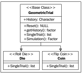
In this section, we define a base class, GeometricTrial, and then redefine the routines so that the Die and Coin classes can be derived from the base class. In doing so, we can demonstrate how inheritance is implemented in the context of an S3 class. Additionally, we respect the idea of encapsulation, which is the principle that an object of a given class should update its own elements using methods from within the class. We explore this issue in greater detail in the section that follows.

We will now rethink the whole class structure. The die and the coin are closely related, and the only difference is the result returned from a single trial. We reimagine the classes to take advantage of the commonalities between the coin and the die. The new class structure is shown in the following diagram:

In addition to the change in the classes, we also change the way in which the classes are defined. In this case, we define functions that will act as constructors for each class. Each constructor will use the class command to append the name of the class to the object's class attribute. As previously mentioned, the class attribute for an object is a vector. When you call the UseMethod command, R will search for a function whose class matches the first element in the vector. If it does not find that function, it looks for a function that matches the second element, and it proceeds until it reaches the last element in the vector. If it does not find anything, it calls the default function. With this in mind, we now examine new definitions of the classes. Rather than manually creating the class, we define functions that will create a list representing the class, append a class name to the class attribute, and then return the list. There are three classes, and we will define one function for each class. The first function is used to define a constructor for an object of the GeometricTrial class:

GeometricTrial <- function()
   {
       # Create the basic data structure - a list that keeps track of
       # a set of trials.

       # Create the basic methods as part of a list to be returned.
       me = list(          
           # Define the history to keep track of the trials.
           history = character(0)
           )

       # Define my class identifier and return the list.
        class(me) <- append(class(me),"GeometricTrial")
       return(me)
   }

Prior to returning the list, the append function is used to add the new class name to the end of the current class attribute. This idea is used in classes that are derived from the GeometricTrial classes as well. The constructor for the Die and Coin classes can now be defined, and both constructors explicitly call the constructor for the parent class, perform any actions associated with the current class, and then append the current class name to the class attribute:

Die <- function()
{
   # Define the object by first calling the constructor for the base class
   me <- GeometricTrial()
   # Add the class name to the end of the list of class names
   class(me) <- append(class(me),"Die")
   return(me)
}

Coin <- function()
{
   # Define the object by calling the constructor for the base class
   me <- GeometricTrial()

   # Add the class name to the end of the list of class names
   class(me) <- append(class(me),"Coin")
   return(me)
}

The GeometricTrial class includes four methods. The reset method behaves exactly like the reset method discussed in the previous section. The getHistory method is an accessor for a data element and is discussed in the following section. We will now discuss the simulation method, and a discussion on the singleTrial method will follow.

The simulation method is used to simulate a single experiment. The history is first cleared, and the singleTrial method is repeatedly called until a successful result is returned. We first define the base simulation function, the default simulation function, and then the simulation function used by the GeometricTrial class, as follows:

simulation <- function(theObject)
   {
       UseMethod("simulation",theObject)
 }

simulation.default <- function(theObject)
   {
       warning("Default simulation method called on unrecognized object.")
       return(theObject)
   }

## Define a method to run a simulation of a geometric trial.
simulation.GeometricTrial = function(theObject)
   {
       theObject <- reset(theObject) # Reset the history
                                       # before the trial.
       repeat
           {
               ## perform a single trial and add it to the history
               thisTrial <- singleTrial(theObject)
               theObject <- appendEvent(theObject,thisTrial$result)
               if(thisTrial$success)
                   {
                      break # The trial resulted in a success. Time
                              # to stop!
                   }
           } # The trial was not a success. Keep going.

       return(theObject)

   }

The effort to define a default function may not appear to be a worthwhile endeavor. However, this practice is generally employed to ensure that the system can responsibly react if the methods you define are called by mistake.

The final step is to define the singleTrial methods. This method is executed by the child classes, Die and Coin. Again, the base and default methods are created. In this case, though, there are also methods for each of the three classes. The base function calls the UseMethod function, which scrolls through the class attribute for the first function to call. We use a method for the GeometricTrial class to demonstrate the order of the calls as well as the NextMethod function. The NextMethod function continues the search in the class attribute and will call the next function based on the class names that follow the current class:

singleTrial.default = function(theObject)
   {
       ## Just generate a default success
       warning("Unrecognized object found for the singleTrial method")
       return(list(result="1",success=TRUE))
   }

singleTrial.GeometricTrial = function(theObject)
   {
       NextMethod("singleTrial",theObject)
   }

singleTrial.Coin = function(theObject)
   {
       ## Perform a single coin flip
       value <- as.character(
           cut(as.integer(1+trunc(runif(1,0,2))),c(0,1,2),labels=c("H","T")))
       return(list(result=value,success=(value=="H")))
   }

singleTrial.Die = function(theObject)
   {
       ## Perform a single die roll
       value <- as.integer(1+trunc(runif(1,0,6)))
       return(list(result=value,success=(value==1)))
   }

With these methods defined and the getHistory method defined in the following section, the class will be complete. Objects of the Coin and Die class can be created, and simulations can be executed, as follows:

> coin <- Coin()
> coin <- simulation(coin)
> getHistory(coin)
[1] H
Levels: H
> coin <- simulation(coin)
> getHistory(coin)
[1] T T H
Levels: H T
> 
> die <- Die()
> die <- simulation(die)
> getHistory(die)
[1] 1
Levels: 1
> die <- simulation(die)
> getHistory(die)
[1] 6 5 5 6 2 1
Levels: 1 2 5 6

Encapsulation

The final method for the getHistory class will now be defined. It is defined in a separate section to stress an important point. An S3 object is generally a basic data structure, such as a vector or a list that has an additional class attribute defined. The functions that are defined for the class react to the class attribute in a predictable way.

One side effect is that every element of an object from a given class is public data. The elements contained within an object can always be accessed. The result is that when programming in R, we must take extra steps to maintain discipline with respect to accessing the data elements maintained by an object. Code that directly accesses data elements within an object may work when first written, but any change to the class constructor risks breaking code in the other methods defined for a class.

With respect to our previous example, we have an accessor, the getHistory method. If we have an object, called oneDie, from the Die class, we can easily get the history using oneDie$history. If we later decide to change the data structure used to store the history, then any code directly accessing this variable is likely to fail.

Instead, we write an accessor method, getHistory, which is designed to return a vector that has the history in the form of a vector of factors. It is important to maintain discipline and only use this method to get a copy of the history. Have a look at the following code:

getHistory <- function(theObject)
   {
       UseMethod("getHistory",theObject)
   }

getHistory.default <- function(theObject)
   {
       return(factor()) # Just return an empty vector of factors
   }

getHistory.GeometricTrial <- function(theObject)
   {
       return(as.factor(theObject$history))
   }

A final note

There is one final note to share about S3 classes. If you have used R, you most likely have used them. Many functions are defined to react according to the class name of their first argument. Have a look at the following diagram:

A common example of this is the plot command. If you type the plot command without arguments, you can see its definition, as follows:

> plot
function (x, y, ...)
UseMethod("plot")
<bytecode: 0x32fdd50>
<environment: namespace:graphics>
>

The plot command will react differently depending on what kind of object you passed to it. If you wish to see what classes the plot command can handle, you can use the methods command to list them:

> methods(plot)
[1] plot.HoltWinters*   plot.TukeyHSD*     plot.acf*    
[4] plot.data.frame*   plot.decomposed.ts* plot.default
[7] plot.dendrogram*   plot.density*       plot.ecdf    
[10] plot.factor*       plot.formula*       plot.function
[13] plot.hclust*       plot.histogram*     plot.isoreg*
[16] plot.lm*           plot.medpolish*     plot.mlm*    
[19] plot.ppr*           plot.prcomp*       plot.princomp*
[22] plot.profile.nls*   plot.spec*         plot.stepfun
[25] plot.stl*           plot.table*         plot.ts      
[28] plot.tskernel*    

   Non-visible functions are asterisked
>

One of the greatest advantages of the S3 class definition is that it is simple to build on what is already available. In the example from the previous section, I would like to have the plot command react appropriately according to whether or not I pass it a class of the type Die or Coin. Assuming that I have the previous classes, Die and Coin, defined, I merely have to define two new plot functions, as follows:

> plot.Die <- function(theDie,theTitle)
+     {
+         plot(theDie$getHistory(),
+             xlab="Value After A Die Roll",ylab="Frequency",
+             main=theTitle)
+     }
>
> plot.Coin <- function(theCoin,theTitle)
+     {
+         plot(theCoin$getHistory(),
+             xlab="Value After Coin Flip",ylab="Frequency",
+             main=theTitle)
+     }
> plot(aCoin,"This Here Trial")
> plot(aDie,"A More Better Trial")

It is common to use this idea to extend a number of commands. Some common examples include the print and the format functions.

Summary

We have explored how to create S3 classes, and we did so in the context of two examples. The first example focused on how to define functions that will react based on the class name of the first argument given to the function. The first example did not make full use of basic object-oriented principles, as it is an attempt to simply introduce the idea of S3 classes. The second example extended the first example to provide a simple example of how inheritance is implemented. It demonstrated how inheritance is implemented in the context of an S3 class. It also provided a demonstration of how encapsulation is implemented under the framework of an S3 class.

One downside to the approach is that there is little type checking. It is possible to make changes to an object that can make it inconsistent with the original definition. When a change is made to an object, no checks are implemented to ensure that an object has the properties that are expected of it.

One way to avoid this issue is to make use of S4 classes. Another advantage is that the S4 approach will look more familiar to those already familiar with object-oriented approaches to programming.

To learn more about R, the following books published by Packt Publishing (https://www.packtpub.com/) are recommended:

• Instant R Starter (https://www.packtpub.com/big-data-and-business-intelligence/instant-r-starter-instant)
• R Object-oriented Programming (https://www.packtpub.com/big-data-and-business-intelligence/r-object-oriented-programming)
• R High Performance Programming (https://www.packtpub.com/application-development/r-high-performance-programming)

Resources for Article:

Further resources on this subject:

• Big Data Analytics[article]
• Data Analytics[article]
• Learning Data Analytics with R and Hadoop[article]