In this article by Dr. Hari M. Kudovely, the author of Learning Bayesian Models with R, we will look at Bayesian inference in depth. The Bayes theorem is the basis for updating beliefs or model parameter values in Bayesian inference, given the observations. In this article, a more formal treatment of Bayesian inference will be given. To begin with, let us try to understand how uncertainties in a real-world problem are treated in Bayesian approach.

(For more resources related to this topic, see here.)

Bayesian view of uncertainty

The classical or frequentist statistics typically take the view that any physical process-generating data containing noise can be modeled by a stochastic model with fixed values of parameters. The parameter values are learned from the observed data through procedures such as maximum likelihood estimate. The essential idea is to search in the parameter space to find the parameter values that maximize the probability of observing the data seen so far. Neither the uncertainty in the estimation of model parameters from data, nor the uncertainty in the model itself that explains the phenomena under study, is dealt with in a formal way. The Bayesian approach, on the other hand, treats all sources of uncertainty using probabilities. Therefore, neither the model to explain an observed dataset nor its parameters are fixed, but they are treated as uncertain variables. Bayesian inference provides a framework to learn the entire distribution of model parameters, not just the values, which maximize the probability of observing the given data. The learning can come from both the evidence provided by observed data and domain knowledge from experts. There is also a framework to select the best model among the family of models suited to explain a given dataset.

Once we have the distribution of model parameters, we can eliminate the effect of uncertainty of parameter estimation in the future values of a random variable predicted using the learned model. This is done by averaging over the model parameter values through marginalization of joint probability distribution.

Consider the joint probability distribution of N random variables again:

This time, we have added one more term, m, to the argument of the probability distribution, in order to indicate explicitly that the parameters are generated by the model m. Then, according to Bayes theorem, the probability distribution of model parameters conditioned on the observed data  and model m is given by:

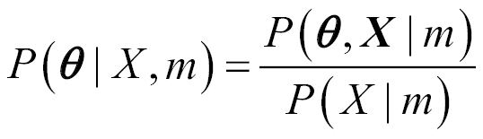
Formally, the term on the LHS of the equation  is called posterior probability distribution. The second term appearing in the numerator of RHS, , is called the prior probability distribution. It represents the prior belief about the model parameters, before observing any data, say, from the domain knowledge. Prior distributions can also have parameters and they are called hyperparameters. The term  is the likelihood of model m explaining the observed data. Since , it can be considered as a normalization constant . The preceding equation can be rewritten in an iterative form as follows:

Here,  represents values of observations that are obtained at time step n,  is the marginal parameter distribution updated until time step n - 1, and  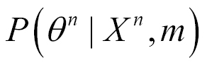is the model parameter distribution updated after seeing the observations  at time step n.

Casting Bayes theorem in this iterative form is useful for online learning and it suggests the following:

• Model parameters can be learned in an iterative way as more and more data or evidence is obtained
• The posterior distribution estimated using the data seen so far can be treated as a prior model when the next set of observations is obtained
• Even if no data is available, one could make predictions based on prior distribution created using the domain knowledge alone

To make these points clear, let's take a simple illustrative example. Consider the case where one is trying to estimate the distribution of the height of males in a given region. The data used for this example is the height measurement in centimeters obtained from M volunteers sampled randomly from the population. We assume that the heights are distributed according to a normal distribution with the mean  and variance :

As mentioned earlier, in classical statistics, one tries to estimate the values of  and  from observed data. Apart from the best estimate value for each parameter, one could also determine an error term of the estimate. In the Bayesian approach, on the other hand,  and  are also treated as random variables. Let's, for simplicity, assume  is a known constant. Also, let's assume that the prior distribution for  is a normal distribution with (hyper) parameters  and . In this case, the expression for posterior distribution of  is given by:

Here, for convenience, we have used the notation  for . It is a simple exercise to expand the terms in the product and complete the squares in the exponential. The resulting expression for the posterior distribution  is given by:

Here,  represents the sample mean. Though the preceding expression looks complex, it has a very simple interpretation. The posterior distribution is also a normal distribution with the following mean:

The variance is as follows:

The posterior mean is a weighted sum of prior mean  and sample mean . As the sample size M increases, the weight of the sample mean increases and that of the prior decreases. Similarly, posterior precision (inverse of the variance) is the sum of the prior precision  and precision of the sample mean :

As M increases, the contribution of precision from observations (evidence) outweighs that from the prior knowledge.

Let's take a concrete example where we consider age distribution with the population mean 5.5 and population standard deviation 0.5. We sample 100 people from this population by using the following R script:

>set.seed(100)
>age_samples <- rnorm(10000,mean = 5.5,sd=0.5)

We can calculate the posterior distribution using the following R function:

>age_mean <- function(n){
mu0 <- 5
sd0 <- 1
mus <- mean(age_samples[1:n])
sds <- sd(age_samples[1:n])
mu_n <- (sd0^2/(sd0^2 + sds^2/n)) * mus + (sds^2/n/(sd0^2 + sds^2/n)) * mu0
mu_n
}
>samp <- c(25,50,100,200,400,500,1000,2000,5000,10000)
>mu <- sapply(samp,age_mean,simplify = "array")
>plot(samp,mu,type="b",col="blue",ylim=c(5.3,5.7),xlab="no of samples",ylab="estimate of mean")
>abline(5.5,0)

One can see that as the number of samples increases, the estimated mean asymptotically approaches the population mean. The initial low value is due to the influence of the prior, which is, in this case, 5.0.

This simple and intuitive picture of how the prior knowledge and evidence from observations contribute to the overall model parameter estimate holds in any Bayesian inference. The precise mathematical expression for how they combine would be different. Therefore, one could start using a model for prediction with just prior information, either from the domain knowledge or the data collected in the past. Also, as new observations arrive, the model can be updated using the Bayesian scheme.

Choosing the right prior distribution

In the preceding simple example, we saw that if the likelihood function has the form of a normal distribution, and when the prior distribution is chosen as normal, the posterior also turns out to be a normal distribution. Also, we could get a closed-form analytical expression for the posterior mean. Since the posterior is obtained by multiplying the prior and likelihood functions and normalizing by integration over the parameter variables, the form of the prior distribution has a significant influence on the posterior. This section gives some more details about the different types of prior distributions and guidelines as to which ones to use in a given context.

There are different ways of classifying prior distributions in a formal way. One of the approaches is based on how much information a prior provides. In this scheme, the prior distributions are classified as Informative, Weakly Informative, Least Informative, and Non-informative. Here, we take more of a practitioner's approach and illustrate some of the important classes of the prior distributions commonly used in practice.

Non-informative priors

Let's start with the case where we do not have any prior knowledge about the model parameters. In this case, we want to express complete ignorance about model parameters through a mathematical expression. This is achieved through what are called non-informative priors. For example, in the case of a single random variable x that can take any value between  and , the non-informative prior for its mean   would be the following:

Here, the complete ignorance of the parameter value is captured through a uniform distribution function in the parameter space. Note that a uniform distribution is not a proper distribution function since its integral over the domain is not equal to 1; therefore, it is not normalizable. However, one can use an improper distribution function for the prior as long as it is multiplied by the likelihood function; the resulting posterior can be normalized.

If the parameter of interest is variance , then by definition it can only take non-negative values. In this case, we transform the variable so that the transformed variable has a uniform probability in the range from  to :

It is easy to show, using simple differential calculus, that the corresponding non-informative distribution function in the original variable  would be as follows:

Another well-known non-informative prior used in practical applications is the Jeffreys prior, which is named after the British statistician Harold Jeffreys. This prior is invariant under reparametrization of  and is defined as proportional to the square root of the determinant of the Fisher information matrix:

Here, it is worth discussing the Fisher information matrix a little bit. If X is a random variable distributed according to , we may like to know how much information observations of X carry about the unknown parameter . This is what the Fisher Information Matrix provides. It is defined as the second moment of the score (first derivative of the logarithm of the likelihood function):

Let's take a simple two-dimensional problem to understand the Fisher information matrix and Jeffreys prior. This example is given by Prof. D. Wittman of the University of California. Let's consider two types of food item: buns and hot dogs.

Let's assume that generally they are produced in pairs (a hot dog and bun pair), but occasionally hot dogs are also produced independently in a separate process. There are two observables such as the number of hot dogs () and the number of buns (), and two model parameters such as the production rate of pairs () and the production rate of hot dogs alone (). We assume that the uncertainty in the measurements of the counts of these two food products is distributed according to the normal distribution, with variance  and , respectively. In this case, the Fisher Information matrix for this problem would be as follows:

In this case, the inverse of the Fisher information matrix would correspond to the covariance matrix:

Subjective priors

One of the key strengths of Bayesian statistics compared to classical (frequentist) statistics is that the framework allows one to capture subjective beliefs about any random variables. Usually, people will have intuitive feelings about minimum, maximum, mean, and most probable or peak values of a random variable. For example, if one is interested in the distribution of hourly temperatures in winter in a tropical country, then the people who are familiar with tropical climates or climatology experts will have a belief that, in winter, the temperature can go as low as 15°C and as high as 27°C with the most probable temperature value being 23°C. This can be captured as a prior distribution through the Triangle distribution as shown here.

The Triangle distribution has three parameters corresponding to a minimum value (a), the most probable value (b), and a maximum value (c). The mean and variance of this distribution are given by:

One can also use a PERT distribution to represent a subjective belief about the minimum, maximum, and most probable value of a random variable. The PERT distribution is a reparametrized Beta distribution, as follows:

Here:

The PERT distribution is commonly used for project completion time analysis, and the name originates from project evaluation and review techniques. Another area where Triangle and PERT distributions are commonly used is in risk modeling.

Often, people also have a belief about the relative probabilities of values of a random variable. For example, when studying the distribution of ages in a population such as Japan or some European countries, where there are more old people than young, an expert could give relative weights for the probability of different ages in the populations. This can be captured through a relative distribution containing the following details:

Here, min and max represent the minimum and maximum values, {values} represents the set of possible observed values, and {weights} represents their relative weights. For example, in the population age distribution problem, these could be the following:

The weights need not have a sum of 1.

Conjugate priors

If both the prior and posterior distributions are in the same family of distributions, then they are called conjugate distributions and the corresponding prior is called a conjugate prior for the likelihood function. Conjugate priors are very helpful for getting get analytical closed-form expressions for the posterior distribution. In the simple example we considered, we saw that when the noise is distributed according to the normal distribution, choosing a normal prior for the mean resulted in a normal posterior. The following table gives examples of some well-known conjugate pairs:

Hierarchical priors

Sometimes, it is useful to define prior distributions for the hyperparameters itself. This is consistent with the Bayesian view that all parameters should be treated as uncertain by using probabilities. These distributions are called hyper-prior distributions. In theory, one can continue this into many levels as a hierarchical model. This is one way of eliciting the optimal prior distributions. For example:

is the prior distribution with a hyperparameter . We could define a prior distribution for  through a second set of equations, as follows:

Here,  is the hyper-prior distribution for the hyperparameter , parametrized by the hyper-hyper-parameter . One can define a prior distribution for in the same way and continue the process forever. The practical reason for formalizing such models is that, at some level of hierarchy, one can define a uniform prior for the hyper parameters, reflecting complete ignorance about the parameter distribution, and effectively truncate the hierarchy. In practical situations, typically, this is done at the second level. This corresponds to, in the preceding example, using a uniform distribution for .

I want to conclude this section by stressing one important point. Though prior distribution has a significant role in Bayesian inference, one need not worry about it too much, as long as the prior chosen is reasonable and consistent with the domain knowledge and evidence seen so far. The reasons are is that, first of all, as we have more evidence, the significance of the prior gets washed out. Secondly, when we use Bayesian models for prediction, we will average over the uncertainty in the estimation of the parameters using the posterior distribution. This averaging is the key ingredient of Bayesian inference and it removes many of the ambiguities in the selection of the right prior.

Estimation of posterior distribution

So far, we discussed the essential concept behind Bayesian inference and also how to choose a prior distribution. Since one needs to compute the posterior distribution of model parameters before one can use the models for prediction, we discuss this task in this section. Though the Bayesian rule has a very simple-looking form, the computation of posterior distribution in a practically usable way is often very challenging. This is primarily because computation of the normalization constant  involves N-dimensional integrals, when there are N parameters. Even when one uses a conjugate prior, this computation can be very difficult to track analytically or numerically. This was one of the main reasons for not using Bayesian inference for multivariate modeling until recent decades. In this section, we will look at various approximate ways of computing posterior distributions that are used in practice.

Maximum a posteriori estimation

Maximum a posteriori (MAP) estimation is a point estimation that corresponds to taking the maximum value or mode of the posterior distribution. Though taking a point estimation does not capture the variability in the parameter estimation, it does take into account the effect of prior distribution to some extent when compared to maximum likelihood estimation. MAP estimation is also called poor man's Bayesian inference.

From the Bayes rule, we have:

Here, for convenience, we have used the notation X for the N-dimensional vector . The last relation follows because the denominator of RHS of Bayes rule is independent of . Compare this with the following maximum likelihood estimate:

The difference between the MAP and ML estimate is that, whereas ML finds the mode of the likelihood function, MAP finds the mode of the product of the likelihood function and prior.

Laplace approximation

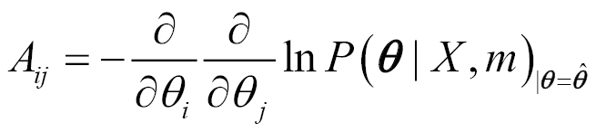
We saw that the MAP estimate just finds the maximum value of the posterior distribution. Laplace approximation goes one step further and also computes the local curvature around the maximum up to quadratic terms. This is equivalent to assuming that the posterior distribution is approximately Gaussian (normal) around the maximum. This would be the case if the amount of data were large compared to the number of parameters: M >> N.

Here, A is an N x N Hessian matrix obtained by taking the derivative of the log of the posterior distribution:

It is straightforward to evaluate the previous expressions at , using the following definition of conditional probability:

We can get an expression for P(X|m) from Laplace approximation that looks like the following:

In the limit of a large number of samples, one can show that this expression simplifies to the following:

The term  is called Bayesian information criterion (BIC) and can be used for model selections or model comparison. This is one of the goodness of fit terms for a statistical model. Another similar criterion that is commonly used is Akaike information criterion (AIC), which is defined by .

Now we will discuss how BIC can be used to compare different models for model selection. In the Bayesian framework, two models such as  and  are compared using the Bayes factor. The definition of the Bayes factor  is the ratio of posterior odds to prior odds that is given by:

Here, posterior odds is the ratio of posterior probabilities of the two models of the given data and prior odds is the ratio of prior probabilities of the two models, as given in the preceding equation. If , model  is preferred by the data and if , model  is preferred by the data.

In reality, it is difficult to compute the Bayes factor because it is difficult to get the precise prior probabilities. It can be shown that, in the large N limit,  can be viewed as a rough approximation to .

Monte Carlo simulations

The two approximations that we have discussed so far, the MAP and Laplace approximations, are useful when the posterior is a very sharply peaked function about the maximum value. Often, in real-life situations, the posterior will have long tails. This is, for example, the case in e-commerce where the probability of the purchasing of a product by a user has a long tail in the space of all products. So, in many practical situations, both MAP and Laplace approximations fail to give good results. Another approach is to directly sample from the posterior distribution. Monte Carlo simulation is a technique used for sampling from the posterior distribution and is one of the workhorses of Bayesian inference in practical applications. In this section, we will introduce the reader to Markov Chain Monte Carlo (MCMC) simulations and also discuss two common MCMC methods used in practice.

As discussed earlier, let  be the set of parameters that we are interested in estimating from the data through posterior distribution. Consider the case of the parameters being discrete, where each parameter has K possible values, that is, . Set up a Markov process with states  and transition probability matrix . The essential idea behind MCMC simulations is that one can choose the transition probabilities in such a way that the steady state distribution of the Markov chain would correspond to the posterior distribution we are interested in. Once this is done, sampling from the Markov chain output, after it has reached a steady state, will give samples of distributed according to the posterior distribution.

Now, the question is how to set up the Markov process in such a way that its steady state distribution corresponds to the posterior of interest. There are two well-known methods for this. One is the Metropolis-Hastings algorithm and the second is Gibbs sampling. We will discuss both in some detail here.

The Metropolis-Hasting algorithm

The Metropolis-Hasting algorithm was one of the first major algorithms proposed for MCMC. It has a very simple concept—something similar to a hill-climbing algorithm in optimization:

1. Let  be the state of the system at time step t.
2. To move the system to another state at time step t + 1, generate a candidate state  by sampling from a proposal distribution . The proposal distribution is chosen in such a way that it is easy to sample from it.
3. Accept the proposal move with the following probability:
4. If it is accepted, = ; if not, .
5. Continue the process until the distribution converges to the steady state.

Here,  is the posterior distribution that we want to simulate. Under certain conditions, the preceding update rule will guarantee that, in the large time limit, the Markov process will approach a steady state distributed according to .

The intuition behind the Metropolis-Hasting algorithm is simple. The proposal distribution  gives the conditional probability of proposing state  to make a transition in the next time step from the current state . Therefore,  is the probability that the system is currently in state  and would make a transition to state  in the next time step. Similarly,  is the probability that the system is currently in state  and would make a transition to state  in the next time step. If the ratio of these two probabilities is more than 1, accept the move. Alternatively, accept the move only with the probability given by the ratio. Therefore, the Metropolis-Hasting algorithm is like a hill-climbing algorithm where one accepts all the moves that are in the upward direction and accepts moves in the downward direction once in a while with a smaller probability. The downward moves help the system not to get stuck in local minima.

Let's revisit the example of estimating the posterior distribution of the mean and variance of the height of people in a population discussed in the introductory section. This time we will estimate the posterior distribution by using the Metropolis-Hasting algorithm. The following lines of R code do this job:

>set.seed(100)
>mu_t <- 5.5
>sd_t <- 0.5
>age_samples <- rnorm(10000,mean = mu_t,sd = sd_t)

>#function to compute log likelihood
>loglikelihood <- function(x,mu,sigma){
   singlell <- dnorm(x,mean = mu,sd = sigma,log = T)
   sumll <- sum(singlell)
   sumll
   }

>#function to compute prior distribution for mean on log scale
>d_prior_mu <- function(mu){
dnorm(mu,0,10,log=T)
}

>#function to compute prior distribution for std dev on log scale
>d_prior_sigma <- function(sigma){
dunif(sigma,0,5,log=T)
}

>#function to compute posterior distribution on log scale
>d_posterior <- function(x,mu,sigma){
loglikelihood(x,mu,sigma) + d_prior_mu(mu) + d_prior_sigma(sigma)
   }
>#function to make transition moves
tran_move <- function(x,dist = .1){
x + rnorm(1,0,dist)
}

>num_iter <- 10000
>posterior <- array(dim = c(2,num_iter))
>accepted <- array(dim=num_iter - 1)
>theta_posterior <-array(dim=c(2,num_iter))

>values_initial <- list(mu = runif(1,4,8),sigma = runif(1,1,5))
>theta_posterior[1,1] <- values_initial$mu
>theta_posterior[2,1] <- values_initial$sigma

>for (t in 2:num_iter){
   #proposed next values for parameters
   theta_proposed               <- c(tran_move(theta_posterior[1,t-1])
               ,tran_move(theta_posterior[2,t-1]))
   p_proposed <- d_posterior(age_samples,mu = theta_proposed[1]
               ,sigma = theta_proposed[2])
   p_prev <-d_posterior(age_samples,mu = theta_posterior[1,t-1]
               ,sigma = theta_posterior[2,t-1])
   eps <- exp(p_proposed - p_prev)

   # proposal is accepted if posterior density is higher w/ theta_proposed
   # if posterior density is not higher, it is accepted with probability eps
   accept <- rbinom(1,1,prob = min(eps,1))
   accepted[t - 1] <- accept
   if (accept == 1){
     theta_posterior[,t] <- theta_proposed
   } else {
     theta_posterior[,t] <- theta_posterior[,t-1]
   }
}

To plot the resulting posterior distribution, we use the sm package in R:

>library(sm)
x <- cbind(c(theta_posterior[1,1:num_iter]),c(theta_posterior[2,1:num_iter]))
xlim <- c(min(x[,1]),max(x[,1]))
ylim <- c(min(x[,2]),max(x[,2]))
zlim <- c(0,max(1))

sm.density(x,
           xlab = "mu",ylab="sigma",
           zlab = " ",zlim = zlim,
           xlim = xlim ,ylim = ylim,col="white")
title("Posterior density")

 The resulting posterior distribution will look like the following figure:

Though the Metropolis-Hasting algorithm is simple to implement for any Bayesian inference problem, in practice it may not be very efficient in many cases. The main reason for this is that, unless one carefully chooses a proposal distribution , there would be too many rejections and it would take a large number of updates to reach the steady state. This is particularly the case when the number of parameters are high. There are various modifications of the basic Metropolis-Hasting algorithms that try to overcome these difficulties. We will briefly describe these when we discuss various R packages for the Metropolis-Hasting algorithm in the following section.

R packages for the Metropolis-Hasting algorithm

There are several contributed packages in R for MCMC simulation using the Metropolis-Hasting algorithm, and here we describe some popular ones.

The mcmc package contributed by Charles J. Geyer and Leif T. Johnson is one of the popular packages in R for MCMC simulations. It has the metrop function for running the basic Metropolis-Hasting algorithm. The metrop function uses a multivariate normal distribution as the proposal distribution.

Sometimes, it is useful to make a variable transformation to improve the speed of convergence in MCMC. The mcmc package has a function named morph for doing this. Combining these two, the function morph.metrop first transforms the variable, does a Metropolis on the transformed density, and converts the results back to the original variable.

Apart from the mcmc package, two other useful packages in R are MHadaptive contributed by Corey Chivers and the Evolutionary Monte Carlo (EMC) algorithm package by Gopi Goswami.

Gibbs sampling

As mentioned before, the Metropolis-Hasting algorithm suffers from the drawback of poor convergence, due to too many rejections, if one does not choose a good proposal distribution. To avoid this problem, two physicists Stuart Geman and Donald Geman proposed a new algorithm. This algorithm is called Gibbs sampling and it is named after the famous physicist J W Gibbs. Currently, Gibbs sampling is the workhorse of MCMC for Bayesian inference.

Let  be the set of parameters of the model that we wish to estimate:

1. Start with an initial state .
2. At each time step, update the components one by one, by drawing from a distribution conditional on the most recent value of rest of the components:

    

    

    

    

3. After N steps, all components of the parameter will be updated.
4. Continue with step 2 until the Markov process converges to a steady state.

 Gibbs sampling is a very efficient algorithm since there are no rejections. However, to be able to use Gibbs sampling, the form of the conditional distributions of the posterior distribution should be known.

R packages for Gibbs sampling

Unfortunately, there are not many contributed general purpose Gibbs sampling packages in R. The gibbs.met package provides two generic functions for performing MCMC in a Naïve way for user-defined target distribution. The first function is gibbs_met. This performs Gibbs sampling with each 1-dimensional distribution sampled by using the Metropolis algorithm, with normal distribution as the proposal distribution. The second function, met_gaussian, updates the whole state with independent normal distribution centered around the previous state. The gibbs.met package is useful for general purpose MCMC on moderate dimensional problems.

Apart from the general purpose MCMC packages, there are several packages in R designed to solve a particular type of machine-learning problems. The GibbsACOV package can be used for one-way mixed-effects ANOVA and ANCOVA models. The lda package performs collapsed Gibbs sampling methods for topic (LDA) models. The stocc package fits a spatial occupancy model via Gibbs sampling. The binomlogit package implements an efficient MCMC for Binomial Logit models. Bmk is a package for doing diagnostics of MCMC output. Bayesian Output Analysis Program (BOA) is another similar package. RBugs is an interface of the well-known OpenBUGS MCMC package. The ggmcmc package is a graphical tool for analyzing MCMC simulation. MCMCglm is a package for generalized linear mixed models and BoomSpikeSlab is a package for doing MCMC for Spike and Slab regression. Finally, SamplerCompare is a package (more of a framework) for comparing the performance of various MCMC packages.

Variational approximation

In the variational approximation scheme, one assumes that the posterior distribution  can be approximated to a factorized form:

Note that the factorized form is also a conditional distribution, so each  can have dependence on other s through the conditioned variable X. In other words, this is not a trivial factorization making each parameter independent. The advantage of this factorization is that one can choose more analytically tractable forms of distribution functions . In fact, one can vary the functions  in such a way that it is as close to the true posterior  as possible. This is mathematically formulated as a variational calculus problem, as explained here.

Let's use some measures to compute the distance between the two probability distributions, such as  and , where . One of the standard measures of distance between probability distributions is the Kullback-Leibler divergence, or KL-divergence for short. It is defined as follows:

The reason why it is called a divergence and not distance is that  is not symmetric with respect to Q and P. One can use the relation  and rewrite the preceding expression as an equation for log P(X):

Here:

Note that, in the equation for ln P(X), there is no dependence on Q on the LHS. Therefore, maximizing  with respect to Q will minimize , since their sum is a term independent of Q. By choosing analytically tractable functions for Q, one can do this maximization in practice. It will result in both an approximation for the posterior and a lower bound for ln P(X) that is the logarithm of evidence or marginal likelihood, since .

Therefore, variational approximation gives us two quantities in one shot. A posterior distribution can be used to make predictions about future observations (as explained in the next section) and a lower bound for evidence can be used for model selection.

How does one implement this minimization of KL-divergence in practice? Without going into mathematical details, here we write a final expression for the solution:

Here,  implies that the expectation of the logarithm of the joint distribution  is taken over all the parameters  except for . Therefore, the minimization of KL-divergence leads to a set of coupled equations; one for each  needs to be solved self-consistently to obtain the final solution. Though the variational approximation looks very complex mathematically, it has a very simple, intuitive explanation. The posterior distribution of each parameter  is obtained by averaging the log of the joint distribution over all the other variables. This is analogous to the Mean Field theory in physics where, if there are N interacting charged particles, the system can be approximated by saying that each particle is in a constant external field, which is the average of fields produced by all the other particles.

We will end this section by mentioning a few R packages for variational approximation. The VBmix package can be used for variational approximation in Bayesian mixture models. A similar package is vbdm used for Bayesian discrete mixture models. The package vbsr is used for variational inference in Spike Regression Regularized Linear Models.

Prediction of future observations

Once we have the posterior distribution inferred from data using some of the methods described already, it can be used to predict future observations. The probability of observing a value Y, given observed data X, and posterior distribution of parameters  is given by:

Note that, in this expression, the likelihood function  is averaged by using the distribution of the parameter given by the posterior . This is, in fact, the core strength of the Bayesian inference. This Bayesian averaging eliminates the uncertainty in estimating the parameter values and makes the prediction more robust.

Summary

In this article, we covered the basic principles of Bayesian inference. Starting with how uncertainty is treated differently in Bayesian statistics compared to classical statistics, we discussed deeply various components of Bayes' rule. Firstly, we learned the different types of prior distributions and how to choose the right one for your problem. Then we learned the estimation of posterior distribution using techniques such as MAP estimation, Laplace approximation, and MCMC simulations.

Resources for Article:

Further resources on this subject:

• Bayesian Network Fundamentals [article]
• Learning Data Analytics with R and Hadoop [article]
• First steps with R [article]