In logistic regression, input features are linearly scaled just as with linear regression; however, the result is then fed as an input to the logistic function. This function provides a nonlinear transformation on its input and ensures that the range of the output, which is interpreted as the probability of the input belonging to class 1, lies in the interval [0,1].

(For more resources related to this topic, see here.)

The form of the logistic function is as follows:

The plot of the logistic function is as follows:

When x = 0, the logistic function takes the value 0.5. As x tends to +∞, the exponential in the denominator vanishes and the function approaches the value 1. As x tends to -∞, the exponential, and hence the denominator, tends to move toward infinity and the function approaches the value 0. Thus, our output is guaranteed to be in the interval [0,1], which is necessary for it to be a probability.

Generalized linear models

Logistic regression belongs to a class of models known as generalized linear models (GLMs). Generalized linear models have three unifying characteristics. The first of these is that they all involve a linear combination of the input features, thus explaining part of their name. The second characteristic is that the output is considered to have an underlying probability distribution belonging to the family of exponential distributions. These include the normal distribution, the Poisson and the binomial distribution. Finally, the mean of the output distribution is related to the linear combination of input features by way of a function, known as the link function. Let's see how this all ties in with logistic regression, which is just one of many examples of a GLM. We know that we begin with a linear combination of input features, so for example, in the case of one input feature, we can build up an x term as follows:

Note that in the case of logistic regression, we are modeling a probability that the output belongs to class 1, rather the output directly as we were in linear regression. As a result, we do not need to model the error term because our output, which is a probability, incorporates nondeterministic aspects of our model, such as measurement uncertainties, directly. Next, we apply the logistic function to this term in order to produce our model's output:

Here, the left term tells us directly that we are computing the probability that our output belongs to class 1 based on our evidence of seeing the values of the input feature X1. For logistic regression, the underlying probability distribution of the output is the Bernoulli distribution. This is the same as the binomial distribution with a single trial and is the distribution we would obtain in an experiment with only two possible outcomes having constant probability, such as a coin flip. The mean of the Bernoulli distribution, μy, is the probability of the (arbitrarily chosen) outcome for success, in this case, class 1. Consequently, the left-hand side in the previous equation is also the mean of our underlying output distribution. For this reason, the function that transforms our linear combination of input features is sometimes known as the mean function, and we just saw that this function is the logistic function for logistic regression. Now, to determine the link function for logistic regression, we can perform some simple algebraic manipulations in order to isolate our linear combination of input features.

The term on the left-hand side is known as the log-odds or logit function and is the link function for logistic regression. The denominator of the fraction inside the logarithm is the probability of the output being class 0 given the data. Consequently, this fraction represents the ratio of probability between class 1 and class 0, which is also known as the odds ratio.

A good reference for logistic regression along with examples of other GLMs such as Poisson regression is Extending the Linear Model with R, Julian J. Faraway, CRC Press.

Interpreting coefficients in logistic regression

Looking at the right-hand side of the last equation, we can see that we have almost exactly the same form as we had for simple linear regression, barring the error term. The fact that we have the logit function on the left-hand side, however, means we cannot interpret our regression coefficients in the same way that we did with linear regression. In logistic regression, a unit increase in feature Xi results in multiplying the odds ratio by an amount, { QUOTE  }. When a coefficient βi is positive, then we multiply the odds ratio by a number greater than 1, so we know that increasing the feature Xi will effectively increase the probability of the output being labeled as class 1. Similarly, increasing a feature with a negative coefficient shifts the balance toward predicting class 0. Finally, note that when we change the value of an input feature, the effect is a multiplication on the odds ratio and not on the model output itself, which we saw is the probability of predicting class 1. In absolute terms, the change in the output of our model as a result of a change in the input is not constant throughout but depends on the current value of our input features. This is, again, different from linear regression, where no matter what the values of the input features, the regression coefficients always represent a fixed increase in the output per unit increase of an input feature.

Assumptions of logistic regression

Logistic regression makes fewer assumptions about the input than linear regression. In particular, the nonlinear transformation of the logistic function means that we can model more complex input-output relationships. We still have a linearity assumption, but in this case, it is between the features and the log-odds. We no longer require a normality assumption for residuals and nor do we need the homoscedastic assumption. On the other hand, our error terms still need to be independent. Strictly speaking, the features themselves no longer need to be independent but in practice, our model will still face issues if the features exhibit a high degree of multicollinearity. Finally, we'll note that just like with unregularized linear regression, feature scaling does not affect the logistic regression model. This means that centering and scaling a particular input feature will simply result in an adjusted coefficient in the output model without any repercussions on the model performance. It turns out that for logistic regression, this is the result of a property known as the invariance property of maximum likelihood, which is the method used to select the coefficients and will be the focus of the next section. It should be noted, however, that centering and scaling features might still be a good idea if they are on very different scales. This is done to assist the optimization procedure during training. In short, we should turn to feature scaling only if we run into model convergence issues.

Maximum likelihood estimation

When we studied linear regression, we found our coefficients by minimizing the sum of squared error terms. For logistic regression, we do this by maximizing the likelihood of the data. The likelihood of an observation is the probability of seeing that observation under a particular model. In our case, the likelihood of seeing an observation X for class 1 is simply given by the probability P(Y=1|X), the form of which was given earlier in this article. As we only have two classes, the likelihood of seeing an observation for class 0 is given by 1 - P(Y=1|X). The overall likelihood of seeing our entire data set of observations is the product of all the individual likelihoods for each data point as we consider our observations to be independently obtained. As the likelihood of each observation is parameterized by the regression coefficients βi, the likelihood function for our entire data set is also, therefore, parameterized by these coefficients. We can express our likelihood function as an equation, as shown in the following equation:

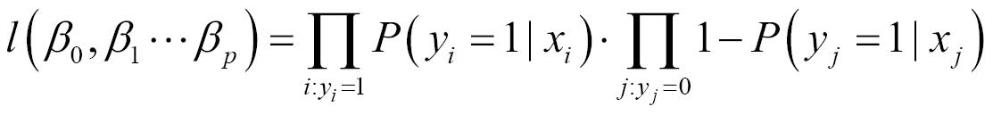
Now, this equation simply computes the probability that a logistic regression model with a particular set of regression coefficients could have generated our training data. The idea is to choose our regression coefficients so that this likelihood function is maximized. We can see that the form of the likelihood function is a product of two large products from the two big π symbols. The first product contains the likelihood of all our observations for class 1, and the second product contains the likelihood of all our observations for class 0. We often refer to the log likelihood of the data, which is computed by taking the logarithm of the likelihood function and using the fact that the logarithm of a product of terms is the sum of the logarithm of each term:

We can simplify this even further using a classic trick to form just a single sum:

To see why this is true, note that for the observations where the actual value of the output variable y is 1, the right term inside the summation is zero, so we are effectively left with the first sum from the previous equation. Similarly, when the actual value of y is 0, then we are left with the second summation from the previous equation. Note that maximizing the likelihood is equivalent to maximizing the log likelihood.

Maximum likelihood estimation is a fundamental technique of parameter fitting and we will encounter it in other models in this book. Despite its popularity, it should be noted that maximum likelihood is not a panacea. Alternative training criteria on which to build a model exist, and there are some well-known scenarios under which this approach does not lead to a good model. Finally, note that the details of the actual optimization procedure that finds the values of the regression coefficients for maximum likelihood are beyond the scope of this book and in general, we can rely on R to implement this for us.

Summary

In this article, we demonstrated why logistic regression is a better way to approach classification problems compared to linear regression with a threshold by showing that the least squares criterion is not the most appropriate criterion to use when trying to separate two classes. It turns out that logistic regression is not a great choice for multiclass settings in general.

To learn more about Predictive Analysis, the following books published by Packt Publishing (https://www.packtpub.com/) are recommended:

• Learning Predictive Analytics with R (https://www.packtpub.com/big-data-and-business-intelligence/learning-predictive-analytics-r)

Resources for Article:

Further resources on this subject:

• Machine learning in practice [article]
• Introduction to Machine Learning with R [article]
• Training and Visualizing a neural network with R [article]