In this article by Anshul Joshi, the author of the book Julia for Data Science, we will learn that data science involves understanding data, gathering data, munging data, taking the meaning out of that data, and then machine learning if needed. Julia is a high-level, high-performance dynamic programming language for technical computing, with syntax that is familiar to users of other technical computing environments.

(For more resources related to this topic, see here.)

The key features offered by Julia are:

• A general purpose high-level dynamic programming language designed to be effective for numerical and scientific computing
• A Low-Level Virtual Machine (LLVM) based Just-in-Time (JIT) compiler that enables Julia to approach the performance of statically-compiled languages like C/C++

What is machine learning?

Generally, when we talk about machine learning, we get into the idea of us fighting wars with intelligent machines that we created but went out of control. These machines are able to outsmart the human race and become a threat to human existence. These theories are nothing but created for our entertainment. We are still very far away from such machines.

So, the question is: what is machine learning? Tom M. Mitchell gave a formal definition-

"A computer program is said to learn from experience E with respect to some class of tasks T and performance measure P if its performance at tasks in T, as measured by P, improves with experience E."

It says that machine learning is teaching computers to generate algorithms using data without programming them explicitly. It transforms data into actionable knowledge. Machine learning has close association with statistics, probability, and mathematical optimization.

As technology grew, there is one thing that grew with it exponentially—data. We have huge amounts of unstructured and structured data growing at a very great pace. Lots of data is generated by space observatories, meteorologists, biologists, fitness sensors, surveys, and so on. It is not possible to manually go through this much amount of data and find patterns or gain insights. This data is very important for scientists, domain experts, governments, health officials, and even businesses. To gain knowledge out of this data, we need self-learning algorithms that can help us in decision making.

Machine learning evolved as a subfield of artificial intelligence, which eliminates the need to manually analyze large amounts of data. Instead of using machine learning, we make data-driven decisions by gaining knowledge using self-learning predictive models. Machine learning has become important in our daily lives. Some common use cases include search engines, games, spam filters, and image recognition. Self-driving cars also use machine learning.

Some basic terminologies used in machine learning:

• Features: Distinctive characteristics of the data point or record
• Training set: This is the dataset that we feed to train the algorithm that helps us to find relationships or build a model
• Testing set: The algorithm generated using the training dataset is tested on the testing dataset to find the accuracy
• Feature vector: An n-dimensional vector that contains the features defining an object
• Sample: An item from the dataset or the record

Uses of machine learning

Machine learning in one way or another is used everywhere. Its applications are endless. Let's discuss some very common use cases:

• E-mail spam filtering: Every major e-mail service provider uses machine learning to filter out spam messages from the Inbox to the Spam folder.
• Predicting storms and natural disasters: Machine learning is used by meteorologists and geologists to predict the natural disasters using weather data, which can help us to take preventive measures.
• Targeted promotions/campaigns and advertising: On social sites, search engines, and maybe in mailboxes, we see advertisements that somehow suit our taste. This is made feasible using machine learning on the data from our past searches, our social profile or the e-mail contents.
• Self-driving cars: Technology giants are currently working on self driving cars. This is made possible using machine learning on the feed of the actual data from human drivers, image and sound processing, and various other factors.
• Machine learning is also used by businesses to predict the market.
• It can also be used to predict the outcomes of elections and the sentiment of voters towards a particular candidate.
• Machine learning is also being used to prevent crime. By understanding the pattern of the different criminals, we can predict a crime that can happen in future and can prevent it.

One case that got a huge amount of attention was of a big retail chain in the United States using machine learning to identify pregnant women. The retailer thought of the strategy to give discounts on multiple maternity products, so that they would become loyal customers and will purchase items for babies which have a high profit margin.

The retailer worked on the algorithm to predict the pregnancy using useful patterns in purchases of different products which are useful for pregnant women.

Once a man approached the retailer and asked for the reason that his teenage daughter is receiving discount coupons for maternity items. The retail chain offered an apology but later the father himself apologized when he got to know that his daughter was indeed pregnant.

This story may or may not be completely true, but retailers indeed analyze their customers' data routinely to find out patterns and for targeted promotions, campaigns, and inventory management.

Machine learning and ethics

Let's see where machine learning is used very frequently:

• Retailers: In the previous example, we mentioned how retail chains use data for machine learning to increase their revenue as well as to retain their customers.
• Spam filtering: E-mails are processed using various machine learning algorithms for spam filtering.
• Targeted advertisements: In our mailbox, social sites, or search engines, we see advertisements of our liking.

These are only some of the actual use cases that are implemented in the world today. One thing that is common between them is the user data.

In the first example, retailers are using the history of transactions done by the user for targeted promotions and campaigns and for inventory management, among other things. Retail giants do this by providing users a loyalty or sign-up card.

In the second example, the e-mail service provider uses trained machine learning algorithms to detect and flag spam. It does by going through the contents of e-mail/attachments and classifying the sender of the e-mail.

In the third example, again the e-mail provider, social network, or search engine will go through our cookies, our profile, or our mails to do the targeted advertising.

In all of these examples, it is mentioned in the terms and conditions of the agreement when we sign up with the retailer, e-mail provider, or social network that the user's data will be used but privacy will not be violated.

It is really important that before using data that is not publicly available, we take the required permissions. Also, our machine learning models shouldn't do discrimination on the basis of region, race, and sex or of any other kind. The data provided should not be used for purposes not mentioned in the agreement or illegal in the region or country of existence.

Machine learning – the process

Machine learning algorithms are trained in keeping with the idea of how the human brain works. They are somewhat similar. Let's discuss the whole process.

The machine learning process can be described in three steps:

• Input
• Abstraction
• Generalization

These three steps are the core of how the machine learning algorithm works. Although the algorithm may or may not be divided or represented in such a way, this explains the overall approach.

• The first step concentrates on what data should be there and what shouldn't. On the basis of that, it gathers, stores, and cleans the data as per the requirements.
• The second step involves that the data be translated to represent the bigger class of data. This is required as we cannot capture everything and our algorithm should not be applicable for only the data that we have.
• The third step focuses on the creation of the model or an action that will use this abstracted data, which will be applicable for the broader mass.

So, what should be the flow of approaching a machine learning problem?

In this particular figure, we see that the data goes through the abstraction process before it can be used to create the machine learning algorithm. This process itself is cumbersome.

The process follows the training of the model, which is fitting the model into the dataset that we have. The computer does not pick up the model on its own, but it is dependent on the learning task. The learning task also includes generalizing the knowledge gained on the data that we don't have yet.

Therefore, training the model is on the data that we currently have and the learning task includes generalization of the model for future data.

It depends on our model how it deduces knowledge from the dataset that we currently have. We need to make such a model that can gather insights into something that wasn't known to us before and how it is useful and can be linked to the future data.

Different types of machine learning

Machine learning is divided mainly into three categories:

• Supervised learning
• Unsupervised learning
• Reinforcement learning

In supervised learning, the model/machine is presented with inputs and the outputs corresponding to those inputs. The machine learns from these inputs and applies this learning in further unseen data to generate outputs.

Unsupervised learning doesn't have the required outputs; therefore it is up to the machine to learn and find patterns that were previously unseen.

In reinforcement learning, the machine continuously interacts with the environment and learns through this process. This includes a feedback loop.

Understanding decision trees

Decision tree is a very good example of divide and conquer. It is one of the most practical and widely used methods for inductive inference. It is a supervised learning method that can be used for both classification and regression. It is non-parametric and its aim is to learn by inferring simple decision rules from the data and create such a model that can predict the value of the target variable.

Before taking a decision, we analyze the probability of the pros and cons by weighing the different options that we have. Let's say we want to purchase a phone and we have multiple choices in the price segment. Each of the phones has something really good, and maybe better than the other. To make a choice, we start by considering the most important feature that we want. And like this, we create a series of features that it has to pass to become the ultimate choice.

In this section, we will learn about:

• Decision trees
• Entropy measures
• Random forests

We will also learn about famous decision tree learning algorithms such as ID3 and C5.0.

Decision tree learning algorithms

There are various decision tree learning algorithms that are actually variations of the core algorithm. The core algorithm is actually a top-down, greedy search through all possible trees.

We are going to discuss two algorithms:

• ID3
• C4.5 and C5.0

The first algorithm, Iterative Dichotomiser 3 (ID3), was developed by Ross Quinlan in 1986. The algorithm proceeds by creating a multiway tree, where it uses greedy search to find each node and the features that can yield maximum information gain for the categorical targets. As trees can grow to the maximum size, which can result in over-fitting of data, pruning is used to make the generalized model.

C4.5 came after ID3 and eliminated the restriction that all features must be categorical. It does this by defining dynamically a discrete attribute based on the numerical variables. This partitions into a discrete set of intervals from the continuous attribute value. C4.5 creates sets of if-then rules from the trained trees of the ID3 algorithm. C5.0 is the latest version; it builds smaller rule sets and uses comparatively lesser memory.

An example

Let's apply what we've learned to create a decision tree using Julia. We will be using the example available for Python on scikit-learn.org and Scikitlearn.jl by Cedric St-Jean.

We will first have to add the required packages:

We will first have to add the required packages:
julia> Pkg.update()
julia> Pkg.add("DecisionTree")
julia> Pkg.add("ScikitLearn")
julia> Pkg.add("PyPlot")

ScikitLearn provides the interface to the much-famous library of machine learning for Python to Julia:

julia> using ScikitLearn
julia> using DecisionTree
julia> using PyPlot

After adding the required packages, we will create the dataset that we will be using in our example:

julia> # Create a random dataset
julia> srand(100)
julia> X = sort(5 * rand(80))
julia> XX = reshape(X, 80, 1)
julia> y = sin(X)
julia> y[1:5:end] += 3 * (0.5 – rand(16))

This will generate a 16-element Array{Float64,1}.

Now we will create instances of two different models. One model is where we will not limit the depth of the tree, and in other model, we will prune the decision tree on the basis of purity:

We will now fit the models to the dataset that we have. We will fit both the models.

This is the first model. Here our decision tree has 25 leaf nodes and a depth of 8.

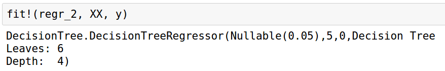
This is the second model. Here we prune our decision tree. This has six leaf nodes and a depth of 4.

Now we will use the models to predict on the test dataset:

julia> # Predict
julia> X_test = 0:0.01:5.0
julia> y_1 = predict(regr_1, hcat(X_test))
julia> y_2 = predict(regr_2, hcat(X_test))

This creates a 501-element Array{Float64,1}.

To better understand the results, let's plot both the models on the dataset that we have:

julia> # Plot the results
julia> scatter(X, y, c="k", label="data")
julia> plot(X_test, y_1, c="g", label="no pruning", linewidth=2)
julia> plot(X_test, y_2, c="r", label="pruning_purity_threshold=0.05", linewidth=2)

julia> xlabel("data")
julia> ylabel("target")
julia> title("Decision Tree Regression")
julia> legend(prop=Dict("size"=>10))

Decision trees can tend to overfit data. It is required to prune the decision tree to make it more generalized. But if we do more pruning than required, then it may lead to an incorrect model. So, it is required that we find the most optimized pruning level.

It is quite evident that the first decision tree overfits to our dataset, whereas the second decision tree model is comparatively more generalized.

Summary

In this article, we learned about machine learning and its uses. Providing computers the ability to learn and improve has far-reaching uses in this world. It is used in predicting disease outbreaks, predicting weather, games, robots, self-driving cars, personal assistants, and lot more. There are three different types of machine learning: supervised learning, unsupervised learning, and reinforcement learning. We also learned about decision trees.

Resources for Article:

Further resources on this subject:

• Specialized Machine Learning Topics [article]
• Basics of Programming in Julia [article]
• More about Julia [article]