In this article by David Julian and Benjamin Baka, author of the book Python Data Structures and Algorithm, we will discern three broad approaches to algorithm design. They are as follows:

• Divide and conquer
• Greedy algorithms
• Dynamic programming

(For more resources related to this topic, see here.)

As the name suggests, the divide and conquer paradigm involves breaking a problem into smaller subproblems, and then in some way combining the results to obtain a global solution. This is a very common and natural problem solving technique and is, arguably, the most used approach to algorithm design.

Greedy algorithms often involve optimization and combinatorial problems; the classic example is applying it to the traveling salesperson problem, where a greedy approach always chooses the closest destination first. This shortest path strategy involves finding the best solution to a local problem in the hope that this will lead to a global solution.

The dynamic programming approach is useful when our subproblems overlap. This is different from divide and conquer. Rather than breaking our problem into independent subproblems, with dynamic programming, intermediate results are cached and can be used in subsequent operations. Like divide and conquer, it uses recursion. However, dynamic programing allows us to compare results at different stages. This can have a performance advantage over divide and conquer for some problems because it is often quicker to retrieve a previously calculated result from memory rather than having to recalculate it.

Recursion and backtracking

Recursion is particularly useful for divide and conquer problems; however, it can be difficult to understand exactly what is happening, since each recursive call is itself spinning off other recursive calls. At the core of a recursive function are two types of cases. Base cases, which tell the recursion when to terminate and recursive cases that call the function they are in. A simple problem that naturally lends itself to a recursive solution is calculating factorials. The recursive factorial algorithm defines two cases—the base case, when n is zero, and the recursive case, when n is greater than zero. A typical implementation is shown in the following code:

def factorial(n):
    #test for a base case
    if n==0:
        return 1
    # make a calculation and a recursive call
    f= n*factorial(n-1)
    print(f)
    return(f)
factorial(4)   

This code prints out the digits 1, 2, 4, 24. To calculate 4!, we require four recursive calls plus the initial parent call. On each recursion, a copy of the methods variables is stored in memory. Once the method returns, it is removed from memory. Here is a way to visualize this process:

It may not necessarily be clear if recursion or iteration is a better solution to a particular problem, after all, they both repeat a series of operations and both are very well suited to divide and conquer approaches to algorithm design. An iteration churns away until the problem is done. Recursion breaks the problem down into smaller chunks and then combines the results. Iteration is often easier for programmers because the control stays local to a loop, whereas recursion can more closely represent mathematical concepts such as factorials. Recursive calls are stored in memory, whereas iterations are not. This creates a tradeoff between processor cycles and memory usage, so choosing which one to use may depend on whether the task is processor or memory intensive. The following table outlines the key differences between recursion and iteration.

Backtracking

Backtracking is a form of recursion that is particularly useful for types of problems such as traversing tree structures where we are presented with a number of options at each node, from which we must choose one. Subsequently, we are presented with a different set of options, and depending on the series of choices made, either a goal state or a dead end is reached. If it is the latter, we mast backtrack to a previous node and traverse a different branch. Backtracking is a divide and conquer method for exhaustive search. Importantly, backtracking prunes branches that cannot give a result.

An example of back tracking is given by the following. Here, we have used a recursive approach to generating all the possible permutations of a given string, s, of a given length n:

def bitStr(n, s):           
    
     if n == 1: return s
     return [ digit + bits for digit in bitStr(1,s)for bits in bitStr(n - 1,s)]

print (bitStr(3,'abc'))

This generates the following output:

Note the double list compression and the two recursive calls within this comprehension. This recursively concatenates each element of the initial sequence, returned when n = 1, with each element of the string generated in the previous recursive call. In this sense, it is backtracking to uncover previously ungenerated combinations. The final string that is returned is all n letter combinations of the initial string.

Divide and conquer – long multiplication

For recursion to be more than just a clever trick, we need to understand how to compare it to other approaches, such as iteration, and to understand when it is use will lead to a faster algorithm. An iterative algorithm that we are all familiar with is the procedure you learned in primary math classes, which was used to multiply two large numbers, that is, long multiplication. If you remember, long multiplication involved iterative multiplying and carry operations followed by a shifting and addition operation. Our aim here is to examine ways to measure how efficient this procedure is and attempt to answer the question, is this the most efficient procedure we can use for multiplying two large numbers together?

In the following figure, we can see that multiplying two 4-digit numbers together requires 16 multiplication operations, and we can generalize to say that an n digit number requires, approximately, n² multiplication operations:

This method of analyzing algorithms, in terms of number of computational primitives such as multiplication and addition, is important because it can give a way to understand the relationship between the time it takes to complete a certain computation and the size of the input to that computation. In particular, we want to know what happens when the input, the number of digits, n, is very large.

Can we do better? A recursive approach

It turns out that in the case of long multiplication, the answer is yes, there are in fact several algorithms for multiplying large numbers that require fewer operations. One of the most well-known alternatives to long multiplication is the Karatsuba algorithm, published in 1962. This takes a fundamentally different approach: rather than iteratively multiplying single digit numbers, it recursively carries out multiplication operation on progressively smaller inputs. Recursive programs call themselves on smaller subset of the input. The first step in building a recursive algorithm is to decompose a large number into several smaller numbers. The most natural way to do this is to simply split the number into halves: the first half comprising the most significant digits and the second half comprising the least significant digits. For example, our four-digit number, 2345, becomes a pair of two digit numbers, 23 and 45. We can write a more general decomposition of any two n-digit numbers x and y using the following, where m is any positive integer less than n.

For x-digit number:

For y-digit number:

So, we can now rewrite our multiplication problem x and y as follows:

When we expand and gather like terms we get the following:

More conveniently, we can write it like this (equation 1):

Here,

It should be pointed out that this suggests a recursive approach to multiplying two numbers since this procedure itself involves multiplication. Specifically, the products ac, ad, bc, and bd all involve numbers smaller than the input number, and so it is conceivable that we could apply the same operation as a partial solution to the overall problem. This algorithm, so far consists of four recursive multiplication steps and it is not immediately clear if it will be faster than the classic long multiplication approach.

What we have discussed so far in regards to the recursive approach to multiplication was well known to mathematicians since the late 19^th century. The Karatsuba algorithm improves on this is by making the following observation. We really only need to know three quantities, z₂ = ac, z₁=ad +bc, and z₀ = bd to solve equation 1. We need to know the values of a, b, c, and d as they contribute to the overall sum and products involved in calculating the quantities z₂, z₁, and z₀. This suggests the possibility that perhaps we can reduce the number of recursive steps. It turns out that this is indeed the situation.

Since the products ac and bd are already in their simplest form, it seems unlikely that we can eliminate these calculations. We can, however, make the following observation:

When we subtract the quantities ac and bd, which we have calculated in the previous recursive step, we get the quantity we need, namely ad + bc:

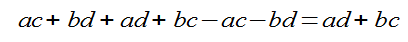
This shows that we can indeed compute the sum of ad and bc without separately computing each of the individual quantities. In summary, we can improve on equation 1 by reducing from four recursive steps to three. These three steps are as follows:

1. Recursively calculate ac.
2. Recursively calculate bd.
3. Recursively calculate (a +b)(c + d) and subtract ac and bd.

The following code shows a Python implementation of the Karatsuba algorithm:

from math import log10 
def karatsuba(x,y):
   
    # The base case for recursion
    if x < 10 or y < 10:
        return x*y    
    
    #sets n, the number of digits in the highest input number
    n = max(int(log10(x)+1), int(log10(y)+1))
    
    # rounds up n/2    
    n_2 = int(math.ceil(n / 2.0))
    #adds 1 if n is uneven
    n = n if n % 2 == 0 else n + 1
    
    #splits the input numbers     
    a, b = divmod(x, 10**n_2)
    c, d = divmod(y, 10**n_2)
    
    #applies the three recursive steps
    ac = karatsuba(a,c)
    bd = karatsuba(b,d)
    ad_bc = karatsuba((a+b),(c+d)) - ac - bd

    #performs the multiplication    
    return (((10**n)*ac) + bd + ((10**n_2)*(ad_bc)))

To satisfy ourselves that this does indeed work, we can run the following test function:

import random
def test():
        for i in range(1000):
            x = random.randint(1,10**5)
            y = random.randint(1,10**5)
            expected = x * y
            result = karatsuba(x, y)
            if result != expected:
                return("failed")                
        return('ok') 

Summary

In this article, we looked at a way to recursively multiply large numbers and also a recursive approach for merge sort. We saw how to use backtracking for exhaustive search and generating strings.

Resources for Article:

Further resources on this subject:

• Python Data Structures [article]
• How is Python code organized [article]
• Algorithm Analysis [article]