This article by Michael Dorman, the author of Learning R for Geospatial Analysis, explores the interplay between vector and raster layers, and the way it is implemented in the raster package. The way rasters and vector layers can be interchanged and queried one according to the other will be demonstrated through examples.

(For more resources related to this topic, see here.)

Creating vector layers from a raster

The opposite operation to rasterization, which has been presented in the previous section, is the creation of vector layers from raster data. The procedure of extracting features of interest out of rasters, in the form of vector layers, is often necessary for analogous reasons underlying rasterization—when the data held in a raster is better represented using a vector layer, within the context of specific subsequent analysis or visualization tasks. Scenarios where we need to create points, lines, and polygons from a raster can all be encountered. In this section, we are going to see an example of each.

Raster-to-points conversion

In raster-to-points conversion, each raster cell center (excluding NA cells) is converted to a point. The resulting point layer has an attribute table with the values of the respective raster cells in it.

Conversion to points can be done with the rasterToPoints function. This function has a parameter named spatial that determines whether the returned object is going to be SpatialPointsDataFrame or simply a matrix holding the coordinates, and the respective cell values (spatial=FALSE, the default value). For our purposes, it is thus important to remember to specify spatial=TRUE.

As an example of a raster, let's create a subset of the raster r, with only layers 1-2, rows 1-3, and columns 1-3:

> u = r[[1:2]][1:3, 1:3, drop = FALSE]

To make the example more instructive, we will place NA in some of the cells and see how this affects the raster-to-points conversion:

> u[2, 3] = NA
> u[[1]][3, 2] = NA

Now, we will apply rasterToPoints to create a SpatialPointsDataFrame object named u_pnt out of u:

> u_pnt = rasterToPoints(u, spatial = TRUE)

Let's visually examine the result we got with the first layer of u serving as the background:

> plot(u[[1]])
> plot(u_pnt, add = TRUE)

The graphical output is shown in the following screenshot:

combining-vector-and-raster-datasets-img-0

We can see that a point has been produced at the center of each raster cell, except for the cell at position (2,3), where we assigned NA to both layers. However, at the (3,2) position, NA has been assigned to only one of the layers (the first one); therefore, a point feature has been generated there nevertheless.

The attribute table of u_pnt has eight rows (since there are eight points) and two columns (corresponding to the raster layers).

> u_pnt@data
layer.1 layer.2
1 0.4242 0.4518
2 0.3995 0.3334
3 0.4190 0.3430
4 0.4495 0.4846
5 0.2925 0.3223
6 0.4998 0.5841
7     NA 0.5841
8 0.7126 0.5086

We can see that the seventh point feature, the one corresponding to the (3,2) raster position, indeed contains an NA value corresponding to layer 1.

Raster-to-contours conversion

Creating points (see the previous section) and polygons (see the next section) from a raster is relatively straightforward. In the former case, points are generated at cell centroids, while in the latter, rectangular polygons are drawn according to cell boundaries. On the other hand, lines can be created from a raster using various different algorithms designed for more specific purposes. Two common procedures where lines are generated based on a raster are constructing contours (lines connecting locations of equal value on the raster) and finding least-cost paths (lines going from one location to another along the easiest route when cost of passage is defined by raster values). In this section, we will see an example of how to create contours (readers interested in least-cost path calculation can refer to the gdistance package, which provides this capability in R).

As an example, we will create contours from the DEM of Haifa (dem). Creating contours can be done using the rasterToContour function. This function accepts a RasterLayer object and returns a SpatialLinesDataFrame object with the contour lines. The rasterToContour function internally uses the base function contourLines, and arguments can be passed to the latter as part of the rasterToContour function call. For example, using the levels parameter, we can specify the breaks where contours will be generated (rather than letting them be determined automatically).

The raster dem consists of elevation values ranging between -14 meters and 541 meters:

> range(dem[], na.rm = TRUE)
[1] -14 541

Therefore, we may choose to generate six contour lines, at 0, 100, 200, …, 500 meter levels:

> dem_contour = rasterToContour(dem, levels = seq(0, 500, 100))

Now, we will plot the resulting SpatialLinesDataFrame object on top of the dem raster:

> plot(dem)

> plot(dem_contour, add = TRUE)

The graphical output is shown in the following screenshot:

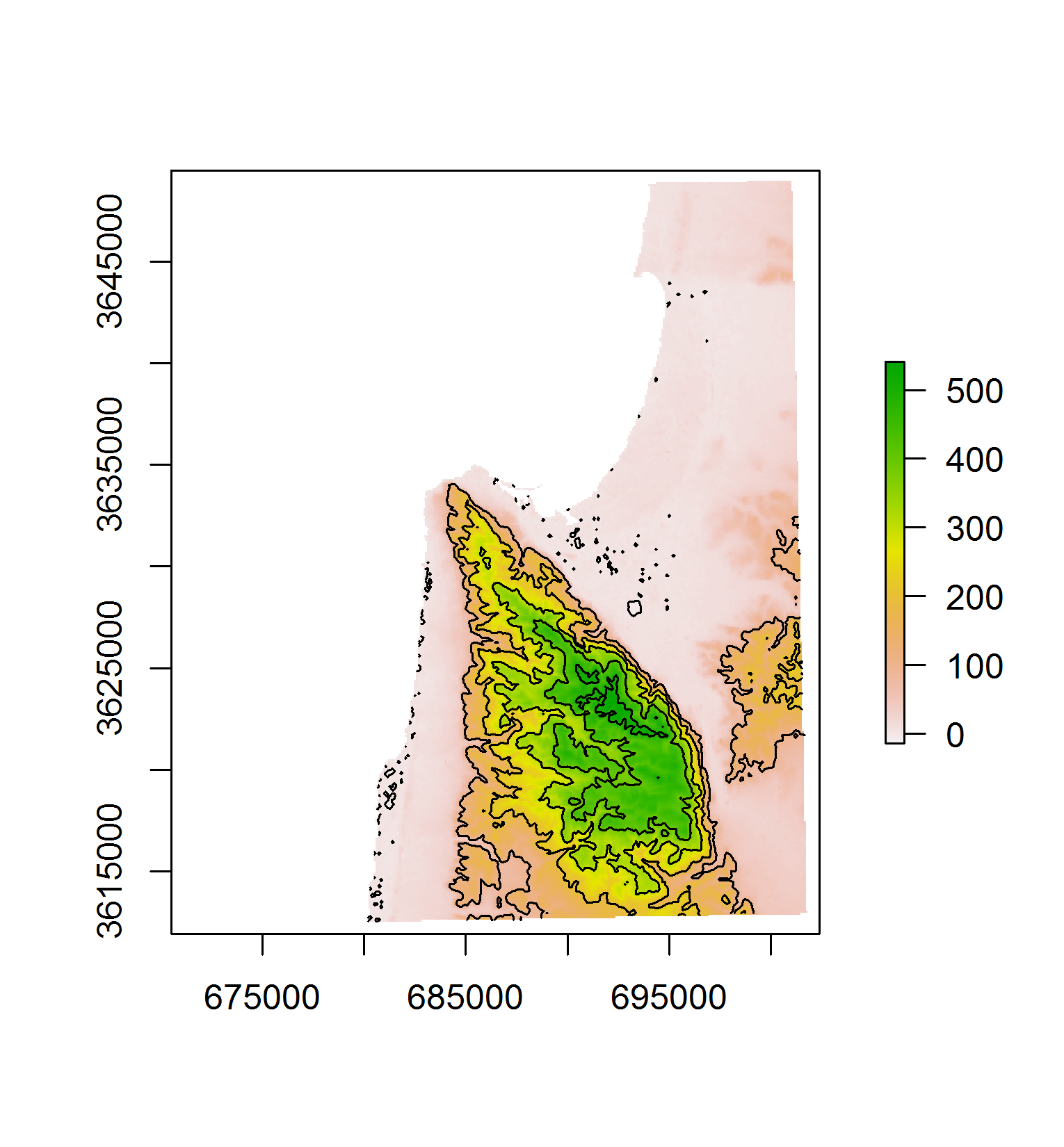
combining-vector-and-raster-datasets-img-1

Mount Carmel is densely covered with elevation contours compared to the plains surrounding it, which are mostly within the 0-100 meter elevation range and thus, have only few a contour lines.

Let's take a look at the attribute table of dem_contour:

> dem_contour@data
   level
C_1     0
C_2   100
C_3   200
C_4   300
C_5   400
C_6   500

Indeed, the layer consists of six line features—one for each break we specified with the levels argument.

Raster-to-polygons conversion

As mentioned previously, raster-to-polygons conversion involves the generation of rectangular polygons in the place of each raster cell (once again, excluding NA cells). Similar to the raster-to-points conversion, the resulting attribute table contains the respective raster values for each polygon created. The conversion to polygons is most useful with categorical rasters when we would like to generate polygons defining certain areas in order to exploit the analysis tools this type of data is associated with (such as extraction of values from other rasters, geometry editing, and overlay).

Creation of polygons from a raster can be performed with a function whose name the reader may have already guessed, rasterToPolygons. A useful option in this function is to immediately dissolve the resulting polygons according to their attribute table values; that is, all polygons having the same value are dissolved into a single feature. This functionality internally utilizes the rgeos package and it can be triggered by specifying dissolve=TRUE.

In our next example, we will visually compare the average NDVI time series of Lahav and Kramim forests (see earlier), based on all of our Landsat (three dates) and MODIS (280 dates) satellite images. In this article, we will only prepare the necessary data by going through the following intermediate steps:

Creating the Lahav and Kramim forests polygonal layer.
Extracting NDVI values from the satellite images.
Creating a data.frame object that can be passed to graphical functions later.

Commencing with the first step, using l_rec_focal_clump, we will first create a polygonal layer holding all NDVI>0.2 patches, then subset only those two polygons corresponding to Lahav and Kramim forests. The former is achieved using rasterToPolygons with dissolve=TRUE, converting the patches in l_rec_focal_clumpto 507 individual polygons in a new SpatialPolygonsDataFrame that we hereby name pol:

> pol = rasterToPolygons(l_rec_focal_clump, dissolve = TRUE)

Plotting pol will show that we have quite a few large patches and many small ones. Since the Lahav and Kramim forests are relatively large, to make things easier, we can omit all polygons with area less than or equal to 1 km2:

> pol$area = gArea(pol, byid = TRUE) / 1000^2

> pol = pol[pol$area > 1, ]

The attribute table shows that we are left with eight polygons, with area sizes of 1-10 km2. The clumps column, by the way, is where the original l_rec_focal_clump raster value (the clump ID) has been kept ("clumps" is the name of the l_rec_focal_clump raster layer from which the values came).

> pol@data
   clumps   area
112     2 1.2231
114   200 1.3284
137   221 1.9314
203   281 9.5274
240   314 6.7842
371   432 2.0007
445     5 10.2159
460     56 1.0998

Let's make a map of pol:

> plotRGB(l_00, r = 3, g = 2, b = 1, stretch = "lin")
> plot(pol, border = "yellow", lty = "dotted", add = TRUE)

The graphical output is shown in the following screenshot:

combining-vector-and-raster-datasets-img-2

The preceding screenshot shows the continuous NDVI>0.2 patches, which are 1 km2 or larger, within the studied area. Two of these, as expected, are the forests we would like to examine. How can we select them? Obviously, we could export pol to a Shapefile and select the features of interest interactively in a GIS software (such as QGIS), then import the result back into R to continue our analysis. The raster package also offers some capabilities for interactive selection (that we do not cover here); for example, a function named click can be used to obtain the properties of the pol features we click in a graphical window such as the one shown in the preceding screenshot. However, given the purpose of this book, we will try to write a code to make the selection automatically without further user input.

To write a code that makes the selection, we must choose a certain criterion (either spatial or nonspatial) that separates the features of interest. In this case, for example, we can see that the pol features we wish to select are those closest to Lahav Kibbutz. Therefore, we can utilize the towns point layer (see earlier) to find the distance of each polygon from Lahav Kibbutz, and select the two most proximate ones.

Using the gDistance function, we will first find out the distances between each polygon in pol and each point in towns:

> dist_towns = gDistance(towns, pol, byid = TRUE)
> dist_towns
             1         2
112 14524.94060 12697.151
114 5484.66695 7529.195
137 3863.12168 5308.062
203   29.48651 1119.090
240 1910.61525 6372.634
371 11687.63594 11276.683
445 12751.21123 14371.268
460 14860.25487 12300.319

The returned matrix, named dist_towns, contains the pairwise distances, with rows corresponding to the pol feature and columns corresponding to the towns feature. Since Lahav Kibbutz corresponds to the first towns feature (column "1"), we can already see that the fourth and fifth pol features (rows "203" and "240") are the most proximate ones, thus corresponding to the Lahav and Kramim forests. We could subset both forests by simply using their IDs—pol[c("203","240"),]. However, as always, we are looking for general code that will select, in this case, the two closest features irrespective of the specific IDs or row indices. For this purpose, we can use the order function, which we have not encountered so far. This function, given a numeric vector, returns the element indices in an increasing order according to element values. For example, applying order to the first column of dist_towns, we can see that the smallest element in this column is in the fourth row, the second smallest is in the fifth row, the third smallest is in the third row, and so on:

> dist_order = order(dist_towns[, 1])
> dist_order
[1] 4 5 3 2 6 7 1 8

We can use this result to select the relevant features of pol as follows:

> forests = pol[dist_order[1:2], ]

The subset SpatialPolygonsDataFrame, named forests, now contains only the two features from pol corresponding to the Lahav and Kramim forests.

> forests@data
   clumps   area
203   281 9.5274
240   314 6.7842

Let's visualize forests within the context of the other data we have by now. We will plot, once again, l_00 as the RGB background and pol on top of it. In addition, we will plot forests (in red) and the location of Lahav Kibbutz (as a red point). We will also add labels for each feature in pol, corresponding to its distance (in meters) from Lahav Kibbutz:

> plotRGB(l_00, r = 3, g = 2, b = 1, stretch = "lin")
> plot(towns[1, ], col = "red", pch = 16, add = TRUE)
> plot(pol, border = "yellow", lty = "dotted", add = TRUE)
> plot(forests, border = "red", lty = "dotted", add = TRUE)
> text(gCentroid(pol, byid = TRUE),
+ round(dist_towns[,1]),
+ col = "White")

The graphical output is shown in the following screenshot:

combining-vector-and-raster-datasets-img-3

The preceding screenshot demonstrates that we did indeed correctly select the features of interest.

We can also assign the forest names to the attribute table of forests, relying on our knowledge that the first feature of forests (ID "203") is larger and more proximate to Lahav Kibbutz and corresponds to the Lahav forest, while the second feature (ID "240") corresponds to Kramim.

> forests$name = c("Lahav", "Kramim")
> forests@data
   clumps   area   name
203   281 9.5274 Lahav
240   314 6.7842 Kramim

We now have a polygonal layer named forests, with two features delineating the Lahav and Kramim forests, named accordingly in the attribute table. In the next section, we will proceed with extracting the NDVI data for these forests.

Summary

In this article, we closed the gap between the two main spatial data types (rasters and vector layers). We now know how to make the conversion from a vector layer to raster and vice versa, and we can transfer the geometry and data components from one data model to another when the need arises. We also saw how raster values can be extracted from a raster according to a vector layer, which is a fundamental step in many analysis tasks involving raster data.