In this article by Alexander Bruy, author of the book, QGIS 2 Cookbook, we will see some of the most common operations related to Digital Elevation Models (DEM).

(For more resources related to this topic, see here.)

Calculating a hillshade layer

A hillshade layer is commonly used to enhance the appearance of a map, and it can be computed from a DEM. This recipe shows how to compute it.

Getting ready

Open the dem_to_prepare.tif layer. This layer contains a DEM in EPSG:4326 CRS and elevation data in feet. These characteristics are unsuitable to runmost terrain analysis algorithms, so we will modify this layer to get a suitable algorithm.

How to do it...

1. In the Processing toolbox, find the Hillshade algorithm and double-click on it to open it, as shown in the following screenshot:

   

2. Select the DEM in the Input layer field.

   Leave the rest of the parameters with their default values.

3. Click on Run to run the algorithm.

The hillshade layer will be added to the QGIS project, as shown in the following screenshot:

How it works...

As in the case of the slope, the algorithm is part of the GDAL library. You will see that the parameters are quite similar to the slope case. This is because the slope is used to compute the hillshade layer. Based on the slope and the aspect of the terrain in each cell, and using the position of the sun defined by the Azimuth and Altitude fields, the algorithm computes the illumination that the cell will receive.

You can try changing the values of these parameters to alter the appearance of the layer.

There's more...

As in the case of slope, there are alternative options to compute the hillshade. The SAGA one in the Processing toolbox has a feature that is worth mentioning.

The SAGA hillshade algorithm contains a field named method. This field is used to select the method used to compute the hillshade value, and the last method available. Raytracing, differs from the other ones. In that it models the real behavior of light, making an analysis that is not local but that uses the full information of the DEM instead. This renders more precise hillshade layers, but the processing time can be notably larger.

Enhancing your map view with a hillshade layer

You can combine the hillshade layer with your other layers to enhance their appearance.

Since you have used a DEM to compute the hillshade layer, it should be already in your QGIS project along with the hillshade itself. However, it will be covered by it since the new layers are produced by the processing. Move it to the top of the layer list, so you can see the DEM (and not the hillshade layer) and style it to something like the following screenshot:

In the Properties dialog of the layer, move to the Transparency section and set the Global transparency value to 50 %, as shown in the following screenshot:

Now you should see the hillshade layer through the DEM, and the combination of both of them will look like the following screenshot:

Analyzing hydrology

A common analysis from a DEM is to compute hydrological elements, such as the channel network or the set of watersheds. This recipe shows the steps to follow to do it.

Getting ready

Open the DEM that we prepared in the previous recipe.

How to do it...

1. In the Processing toolbox, find the Fill sinks algorithm and double-click on it to open that:

   

   Unlock access to the largest independent learning library in Tech for FREE!

   Get unlimited access to 7500+ expert-authored eBooks and video courses covering every tech area you can think of.

   Renews at AU $19.99/month. Cancel anytime

   START FREE TRIAL
2. Select the DEM in the DEM field and run the algorithm. It will generate a new filtered DEM layer. From now on, we will just use this DEM in the recipe, but not the original one.
3. Open the Catchment Area in and select the filtered DEM in the Elevation field:

   

4. Run the algorithm. It will generate a Catchment Area layer.
5. Open the Channel network algorithm and fill it, as shown in the following screenshot:

   

6. Run the algorithm. It will extract the channel network from the DEM based on Catchment Area and generate it as both raster and vector layer.
7. Open the Watershed basins algorithm and fill it, as shown in the following screenshot:

   

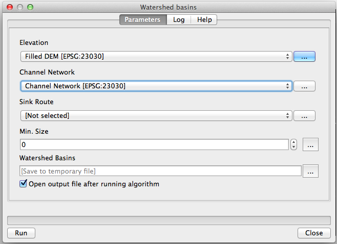
8. Run the algorithm. It will generate a raster layer with the watersheds calculated from the DEM and the channel network. Each watershed is a hydrological unit that represents the area that flows into a junction defined by the channel network:

   

How it works...

Starting from the DEM, the preceding described steps follow a typical workflow for hydrological analysis:

• First, the sinks are removed. This is a required preparation whenever you plan to do hydrological analysis. The DEM might contain sinks where a flow direction cannot be computed, which represents a problem in order to model the movement of water across those cells. Removing them solves this problem.
• The catchment area is computed from the DEM. The values in the catchment area layer represent the area upstream of each cell. That is, the total area in which, if water is dropped, it will eventually reach the cell.
• Cells with high values of catchment area will likely contain a river, whereas cell with lower values will have the overland flow. By setting a threshold on the catchment area values, we can separate the river cells (those above the threshold) from the remaining ones and extract the channel network.
• Finally, we compute the watersheds associated with each junction in the channel network extracted in the last step.

There's more...

The key parameter in the preceding workflow is the catchment area threshold. If a larger threshold is used, fewer cells will be considered as river cells, and the resulting channel network will be sparser. Because the watersheds are computed based on the channel network, it will result in a lower number of watersheds.

You can try yourself with different values of the catchment area threshold. Here, you can see the result for threshold equal to 10,00,000 and 5,00,00,000. The following screenshot shows the result of threshold equal to 10,00,000:

The following screenshot shows the result of threshold equal to 5,00,00,000:

Note that in the previous case, with a higher threshold value, there is only one single watershed in the resulting layer.

The threshold values are expressed in the units of the catchment area, which, because the cell size is assumed to be in meters, are in square meters.

Calculating a topographic index

Because the topography defines and influences most of the processes that take place in a given terrain, the DEM can be used to extract many different parameters that give us information about those processes. This recipe shows to calculate a popular one named the Topographic Wetness Index, which estimates the soil wetness based on the topography.

Getting ready

Open the DEM that we prepared in the Calculating a hillshade layer recipe.

How to do it...

1. Calculate a slope layer using the Slope, Aspect, and Curvature algorithm from the Processing toolbox.
2. Calculate a catchment area layer using the Catchment Area algorithm from the Processing toolbox. Note that you must use a sinkless DEM, as the DEM that we generated in the previous recipe with the Fill sinks algorithm.
3. Open the Topographic Wetness Index algorithm from the Processing toolbox and fill it, as shown in the following screenshot:

   

4. Run the algorithm. It will create a layer with the Topographic Wetness Index field indicating the soil wetness in each cell:

   

How it works...

The index combines slope and catchment area, two parameters that influence the soil wetness. If the catchment area value is high, it means more water will flow into the cell thus increasing its soil wetness. A low value of slope will have a similar effect because the water that flows into the cell will not flow out of it quickly.

The algorithm expects the slope to be expressed in radians. That's the reason why the Slope, Aspect, and Curvature algorithm has to be used because it produces its slope output in radians. The Slope algorithm that you will also find, which is based on the GDAL library, creates a slope layer with values expressed in degrees. You can use that layer if you convert its units by using the raster calculator.

There's more...

Other indices based on the same input layers can be found in different algorithm in the Processing toolbox. The Stream Power Index and the LS factor fields use the slope and catchment area as inputs as well and can be related to potential erosion.

Summary

In this article, we saw the working of the hillshade layer and a topographic index along with their calculation technique. We also saw how to analyze hydrology.

Resources for Article:

Further resources on this subject:

• Identifying the Best Places [article]
• Style Management in QGIS [article]
• Geolocating photos on the map [article]