In this article by Balázs Márkus, coauthor of the book Mastering R for Quantitative Finance, you will learn about pricing and life of Double-no-touch (DNT) option.

(For more resources related to this topic, see here.)

A Double-no-touch (DNT) option is a binary option that pays a fixed amount of cash at expiry. Unfortunately, the fExoticOptions package does not contain a formula for this option at present. We will show two different ways to price DNTs that incorporate two different pricing approaches. In this section, we will call the function dnt1, and for the second approach, we will use dnt2 as the name for the function.

Hui (1996) showed how a one-touch double barrier binary option can be priced. In his terminology, "one-touch" means that a single trade is enough to trigger the knock-out event, and "double barrier" binary means that there are two barriers and this is a binary option. We call this DNT as it is commonly used on the FX markets. This is a good example for the fact that many popular exotic options are running under more than one name. In Haug (2007a), the Hui-formula is already translated into the generalized framework. S, r, b, s, and T have the same meaning. K means the payout (dollar amount) while L and U are the lower and upper barriers.

Where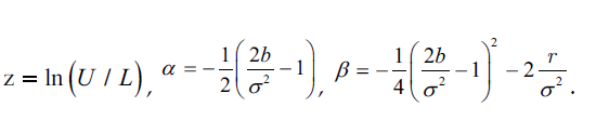

Implementing the Hui (1996) function to R starts with a big question mark: what should we do with an infinite sum? How high a number should we substitute as infinity? Interestingly, for practical purposes, small number like 5 or 10 could often play the role of infinity rather well. Hui (1996) states that convergence is fast most of the time. We are a bit skeptical about this since a will be used as an exponent. If b is negative and sigma is small enough, the (S/L)a part in the formula could turn out to be a problem.

First, we will try with normal parameters and see how quick the convergence is:

dnt1 <- function(S, K, U, L, sigma, T, r, b, N = 20, ploterror = FALSE){
   if ( L > S | S > U) return(0)
   Z <- log(U/L)
   alpha <- -1/2*(2*b/sigma^2 - 1)
   beta <- -1/4*(2*b/sigma^2 - 1)^2 - 2*r/sigma^2
   v <- rep(0, N)
   for (i in 1:N)
       v[i] <- 2*pi*i*K/(Z^2) * (((S/L)^alpha - (-1)^i*(S/U)^alpha ) /
           (alpha^2+(i*pi/Z)^2)) * sin(i*pi/Z*log(S/L)) *
             exp(-1/2 * ((i*pi/Z)^2-beta) * sigma^2*T)
   if (ploterror) barplot(v, main = "Formula Error");
   sum(v)
}
print(dnt1(100, 10, 120, 80, 0.1, 0.25, 0.05, 0.03, 20, TRUE))

The following screenshot shows the result of the preceding code:

The Formula Error chart shows that after the seventh step, additional steps were not influencing the result. This means that for practical purposes, the infinite sum can be quickly estimated by calculating only the first seven steps. This looks like a very quick convergence indeed. However, this could be pure luck or coincidence.

What about decreasing the volatility down to 3 percent? We have to set N as 50 to see the convergence:

print(dnt1(100, 10, 120, 80, 0.03, 0.25, 0.05, 0.03, 50, TRUE))

The preceding command gives the following output:

Not so impressive? 50 steps are still not that bad. What about decreasing the volatility even lower? At 1 percent, the formula with these parameters simply blows up. First, this looks catastrophic; however, the price of a DNT was already 98.75 percent of the payout when we used 3 percent volatility. Logic says that the DNT price should be a monotone-decreasing function of volatility, so we already know that the price of the DNT should be worth at least 98.75 percent if volatility is below 3 percent.

Another issue is that if we choose an extreme high U or extreme low L, calculation errors emerge. However, similar to the problem with volatility, common sense helps here too; the price of a DNT should increase if we make U higher or L lower.

There is still another trick. Since all the problem comes from the a parameter, we can try setting b as 0, which will make a equal to 0.5. If we also set r to 0, the price of a DNT converges into 100 percent as the volatility drops.

Anyway, whenever we substitute an infinite sum by a finite sum, it is always good to know when it will work and when it will not. We made a new code that takes into consideration that convergence is not always quick. The trick is that the function calculates the next step as long as the last step made any significant change. This is still not good for all the parameters as there is no cure for very low volatility, except that we accept the fact that if implied volatilities are below 1 percent, than this is an extreme market situation in which case DNT options should not be priced by this formula:

dnt1 <- function(S, K, U, L, sigma, Time, r, b) {
 if ( L > S | S > U) return(0)
 Z <- log(U/L)
 alpha <- -1/2*(2*b/sigma^2 - 1)
 beta <- -1/4*(2*b/sigma^2 - 1)^2 - 2*r/sigma^2
 p <- 0
 i <- a <- 1
 while (abs(a) > 0.0001){
   a <- 2*pi*i*K/(Z^2) * (((S/L)^alpha - (-1)^i*(S/U)^alpha ) / 
      (alpha^2 + (i *pi / Z)^2) ) * sin(i * pi / Z * log(S/L)) * 
        exp(-1/2*((i*pi/Z)^2-beta) * sigma^2 * Time)
   p <- p + a
   i <- i + 1
 }
 p
}

Now that we have a nice formula, it is possible to draw some DNT-related charts to get more familiar with this option. Later, we will use a particular AUDUSD DNT option with the following parameters: L equal to 0.9200, U equal to 0.9600, K (payout) equal to USD 1 million, T equal to 0.25 years, volatility equal to 6 percent,
r_AUD equal to 2.75 percent, r_USD equal to 0.25 percent, and b equal to -2.5 percent. We will calculate and plot all the possible values of this DNT from 0.9200
to 0.9600; each step will be one pip (0.0001), so we will use 2,000 steps.

The following code plots a graph of price of underlying:

x <- seq(0.92, 0.96, length = 2000)
y <- z <- rep(0, 2000)
for (i in 1:2000){
   y[i] <- dnt1(x[i], 1e6, 0.96, 0.92, 0.06, 0.25, 0.0025, -0.0250)
   z[i] <- dnt1(x[i], 1e6, 0.96, 0.92, 0.065, 0.25, 0.0025, -0.0250)
}
matplot(x, cbind(y,z), type = "l", lwd = 2, lty = 1,
   main = "Price of a DNT with volatility 6% and 6.5%
", cex.main = 0.8, xlab = "Price of underlying" )

The following output is the result of the preceding code:

It can be clearly seen that even a small change in volatility can have a huge impact on the price of a DNT. Looking at this chart is an intuitive way to find that vega must be negative. Interestingly enough even just taking a quick look at this chart can convince us that the absolute value of vega is decreasing if we are getting closer to the barriers.

Most end users think that the biggest risk is when the spot is getting close to the trigger. This is because end users really think about binary options in a binary way. As long as the DNT is alive, they focus on the positive outcome. However, for a dynamic hedger, the risk of a DNT is not that interesting when the value of the DNT is already small.

It is also very interesting that since the T-Bill price is independent of the volatility and since the DNT + DOT = T-Bill equation holds, an increasing volatility will decrease the price of the DNT by the exact same amount just like it will increase the price of the DOT. It is not surprising that the vega of the DOT should be the exact mirror of the DNT.

We can use the GetGreeks function to estimate vega, gamma, delta, and theta.
For gamma we can use the GetGreeks function in the following way:

GetGreeks <- function(FUN, arg, epsilon,...) {
   all_args1 <- all_args2 <- list(...)
   all_args1[[arg]] <- as.numeric(all_args1[[arg]] + epsilon)
   all_args2[[arg]] <- as.numeric(all_args2[[arg]] - epsilon)
   (do.call(FUN, all_args1) -
       do.call(FUN, all_args2)) / (2 * epsilon)
}
Gamma <- function(FUN, epsilon, S, ...) {
   arg1 <- list(S, ...)
   arg2 <- list(S + 2 * epsilon, ...)
   arg3 <- list(S - 2 * epsilon, ...)
   y1 <- (do.call(FUN, arg2) - do.call(FUN, arg1)) / (2 * epsilon)
   y2 <- (do.call(FUN, arg1) - do.call(FUN, arg3)) / (2 * epsilon)
  (y1 - y2) / (2 * epsilon)
}
x = seq(0.9202, 0.9598, length = 200)
delta <- vega <- theta <- gamma <- rep(0, 200)
 
for(i in 1:200){
 delta[i] <- GetGreeks(FUN = dnt1, arg = 1, epsilon = 0.0001, 
   x[i], 1000000, 0.96, 0.92, 0.06, 0.5, 0.02, -0.02)
 vega[i] <-   GetGreeks(FUN = dnt1, arg = 5, epsilon = 0.0005, 
   x[i], 1000000, 0.96, 0.92, 0.06, 0.5, 0.0025, -0.025)
 theta[i] <- - GetGreeks(FUN = dnt1, arg = 6, epsilon = 1/365, 
   x[i], 1000000, 0.96, 0.92, 0.06, 0.5, 0.0025, -0.025)
 gamma[i] <- Gamma(FUN = dnt1, epsilon = 0.0001, S = x[i], K = 
   1e6, U = 0.96, L = 0.92, sigma = 0.06, Time = 0.5, r = 0.02, b = -0.02)
}
 
windows()
plot(x, vega, type = "l", xlab = "S",ylab = "", main = "Vega")

The following chart is the result of the preceding code:

After having a look at the value chart, the delta of a DNT is also very close to intuitions; if we are coming close to the higher barrier, our delta gets negative, and if we are coming closer to the lower barrier, the delta gets positive as follows:

windows()
plot(x, delta, type = "l", xlab = "S",ylab = "", main = "Delta")

This is really a non-convex situation; if we would like to do a dynamic delta hedge, we will lose money for sure. If the spot price goes up, the delta of the DNT decreases, so we should buy some AUDUSD as a hedge. However, if the spot price goes down, we should sell some AUDUSD. Imagine a scenario where AUDUSD goes up 20 pips in the morning and then goes down 20 pips in the afternoon. For a dynamic hedger, this means buying some AUDUSD after the price moved up and selling this very same amount after the price comes down.

The changing of the delta can be described by the gamma as follows:

windows()
plot(x, gamma, type = "l", xlab = "S",ylab = "", main = "Gamma")

Negative gamma means that if the spot goes up, our delta is decreasing, but if the spot goes down, our delta is increasing. This doesn't sound great. For this inconvenient non-convex situation, there is some compensation, that is, the value of theta is positive. If nothing happens, but one day passes, the DNT will automatically worth more.

Here, we use theta as minus 1 times the partial derivative, since if (T-t) is the time left, we check how the value changes as t increases by one day:

windows()
plot(x, theta, type = "l", xlab = "S",ylab = "", main = "Theta")

The more negative the gamma, the more positive our theta. This is how time compensates for the potential losses generated by the negative gamma.

Risk-neutral pricing also implicates that negative gamma should be compensated by a positive theta. This is the main message of the Black-Scholes framework for vanilla options, but this is also true for exotics. See Taleb (1997) and Wilmott (2006).

We already introduced the Black-Scholes surface before; now, we can go into more detail. This surface is also a nice interpretation of how theta and delta work. It shows the price of an option for different spot prices and times to maturity, so the slope of this surface is the theta for one direction and delta for the other. The code for this is as follows:

BS_surf <- function(S, Time, FUN, ...) {
 n <- length(S)
 k <- length(Time) 
 m <- matrix(0, n, k)
 for (i in 1:n) {
   for (j in 1:k) {
     l <- list(S = S[i], Time = Time[j], ...)
     m[i,j] <- do.call(FUN, l)
     }
 }
 persp3D(z = m, xlab = "underlying", ylab = "Time",
    zlab = "option price", phi = 30, theta = 30, bty = "b2")
}
BS_surf(seq(0.92,0.96,length = 200), seq(1/365, 1/48, length = 200),
 dnt1, K = 1000000, U = 0.96, L = 0.92, r = 0.0025, b = -0.0250,
    sigma = 0.2)

The preceding code gives the following output:

We can see what was already suspected; DNT likes when time is passing and the spot is moving to the middle of the (L,U) interval.

Another way to price the Double-no-touch option

Static replication is always the most elegant way of pricing. The no-arbitrage argument will let us say that if, at some time in the future, two portfolios have the same value for sure, then their price should be equal any time before this. We will show how double-knock-out (DKO) options could be used to build a DNT. We will need to use a trick; the strike price could be the same as one of the barriers. For a DKO call, the strike price should be lower than the upper barrier because if the strike price is not lower than the upper barrier, the DKO call would be knocked out before it could become in-the-money, so in this case, the option would be worthless as nobody can ever exercise it in-the-money. However, we can choose the strike price to be equal to the lower barrier. For a put, the strike price should be higher than the lower barrier, so why not make it equal to the upper barrier. This way, the DKO call and DKO put option will have a very convenient feature; if they are still alive, they will both expiry in-the-money.

Now, we are almost done. We just have to add the DKO prices, and we will get a DNT that has a payout of (U-L) dollars. Since DNT prices are linear in the payout, we only have to multiply the result by K*(U-L):

dnt2 <- function(S, K, U, L, sigma, T, r, b) {
 
   a <- DoubleBarrierOption("co", S, L, L, U, T, r, b, sigma, 0,
       0,title = NULL, description = NULL)
   z <- a@price
   b <- DoubleBarrierOption("po", S, U, L, U, T, r, b, sigma, 0,
       0,title = NULL, description = NULL)
   y <- b@price
   (z + y) / (U - L) * K
}

Now, we have two functions for which we can compare the results:

dnt1(0.9266, 1000000, 0.9600, 0.9200, 0.06, 0.25, 0.0025, -0.025)
[1] 48564.59
 
dnt2(0.9266, 1000000, 0.9600, 0.9200, 0.06, 0.25, 0.0025, -0.025)
[1] 48564.45

For a DNT with a USD 1 million contingent payout and an initial market value of over 48,000 dollars, it is very nice to see that the difference in the prices is only 14 cents. Technically, however, having a second pricing function is not a big help since low volatility is also an issue for dnt2.

We will use dnt1 for the rest of the article.

The life of a Double-no-touch option – a simulation

How has the DNT price been evolving during the second quarter of 2014?
We have the open-high-low-close type time series with five minute frequency for AUDUSD, so we know all the extreme prices:

d <- read.table("audusd.csv", colClasses = c("character", rep("numeric",5)), sep = ";", header = TRUE)
underlying <- as.vector(t(d[, 2:5]))
t <- rep( d[,6], each = 4)
n <- length(t)
option_price <- rep(0, n)
 
for (i in 1:n) {
 option_price[i] <- dnt1(S = underlying[i], K = 1000000, 
    U = 0.9600, L = 0.9200, sigma = 0.06, T = t[i]/(60*24*365), 
      r = 0.0025, b = -0.0250)
}
a <- min(option_price)
b <- max(option_price)
option_price_transformed = (option_price - a) * 0.03 / (b - a) + 0.92
 
par(mar = c(6, 3, 3, 5))
matplot(cbind(underlying,option_price_transformed), type = "l",
   lty = 1, col = c("grey", "red"),
   main = "Price of underlying and DNT",
   xaxt = "n", yaxt = "n", ylim = c(0.91,0.97),
   ylab = "", xlab = "Remaining time")
abline(h = c(0.92, 0.96), col = "green")
axis(side = 2, at = pretty(option_price_transformed),
   col.axis = "grey", col = "grey")
axis(side = 4, at = pretty(option_price_transformed),
   labels = round(seq(a/1000,1000,length = 7)), las = 2,
   col = "red", col.axis = "red")
axis(side = 1, at = seq(1,n, length=6),
   labels = round(t[round(seq(1,n, length=6))]/60/24))

The following is the output for the preceding code:

The price of a DNT is shown in red on the right axis (divided by 1000), and the actual AUDUSD price is shown in grey on the left axis. The green lines are the barriers of 0.9200 and 0.9600. The chart shows that in 2014 Q2, the AUDUSD currency pair was traded inside the (0.9200; 0.9600) interval; thus, the payout of the DNT would have been USD 1 million. This DNT looks like a very good investment; however, reality is just one trajectory out of an a priori almost infinite set. It could have happened differently. For example, on May 02, 2014, there were still 59 days left until expiry, and AUDUSD was traded at 0.9203, just three pips away from the lower barrier. At this point, the price of this DNT was only USD 5,302 dollars which is shown in the following code:

dnt1(0.9203, 1000000, 0.9600, 0.9200, 0.06, 59/365, 0.0025, -0.025)
[1] 5302.213

Compare this USD 5,302 to the initial USD 48,564 option price!

In the following simulation, we will show some different trajectories. All of them start from the same 0.9266 AUDUSD spot price as it was on the dawn of April 01, and we will see how many of them stayed inside the (0.9200; 0.9600) interval. To make it simple, we will simulate geometric Brown motions by using the same 6 percent volatility as we used to price the DNT:

library(matrixStats)
DNT_sim <- function(S0 = 0.9266, mu = 0, sigma = 0.06, U = 0.96,
 L = 0.92, N = 5) {
   dt <- 5 / (365 * 24 * 60)
   t <- seq(0, 0.25, by = dt)
   Time <- length(t)
 
   W <- matrix(rnorm((Time - 1) * N), Time - 1, N)
   W <- apply(W, 2, cumsum)
   W <- sqrt(dt) * rbind(rep(0, N), W)
   S <- S0 * exp((mu - sigma^2 / 2) * t + sigma * W )
   option_price <- matrix(0, Time, N)
 
   for (i in 1:N)
       for (j in 1:Time)
         option_price[j,i] <- dnt1(S[j,i], K = 1000000, U, L, sigma,
              0.25-t[j], r = 0.0025,
               b = -0.0250)*(min(S[1:j,i]) > L & max(S[1:j,i]) < U)
 
   survivals <- sum(option_price[Time,] > 0)
   dev.new(width = 19, height = 10)
 
   par(mfrow = c(1,2))
   matplot(t,S, type = "l", main = "Underlying price",
       xlab = paste("Survived", survivals, "from", N), ylab = "")
   abline( h = c(U,L), col = "blue")
   matplot(t, option_price, type = "l", main = "DNT price",
       xlab = "", ylab = "")}
set.seed(214)
system.time(DNT_sim())

The following is the output for the preceding code:

Here, the only surviving trajectory is the red one; in all other cases, the DNT hits either the higher or the lower barrier. The line set.seed(214) grants that this simulation will look the same anytime we run this. One out of five is still not that bad; it would suggest that for an end user or gambler who does no dynamic hedging, this option has an approximate value of 20 percent of the payout (especially since the interest rates are low, the time value of money is not important).

However, five trajectories are still too few to jump to such conclusions. We should check the DNT survivorship ratio for a much higher number of trajectories.

The ratio of the surviving trajectories could be a good estimator of the a priori real-world survivorship probability of this DNT; thus, the end user value of it. Before increasing N rapidly, we should keep in mind how much time this simulation took. For my computer, it took 50.75 seconds for N = 5, and 153.11 seconds for N = 15.

The following is the output for N = 15:

Now, 3 out of 15 survived, so the estimated survivorship ratio is still 3/15, which is equal to 20 percent. Looks like this is a very nice product; the price is around 5 percent of the payout, while 20 percent is the estimated survivorship ratio. Just out of curiosity, run the simulation for N equal to 200. This should take about 30 minutes.

The following is the output for N = 200:

The results are shocking; now, only 12 out of 200 survive, and the ratio is only 6 percent! So to get a better picture, we should run the simulation for a larger N.

The movie Whatever Works by Woody Allen (starring Larry David) is 92 minutes long; in simulation time, that is N = 541. For this N = 541, there are only 38 surviving trajectories, resulting in a survivorship ratio of 7 percent.

What is the real expected survivorship ratio? Is it 20 percent, 6 percent, or 7 percent? We simply don't know at this point. Mathematicians warn us that the law of large numbers requires large numbers, where large is much more than 541, so it would be advisable to run this simulation for as large an N as time allows. Of course, getting a better computer also helps to do more N during the same time. Anyway, from this point of view, Hui's (1996) relatively fast converging DNT pricing formula gets some respect.

Summary

We started this article by introducing exotic options. In a brief theoretical summary, we explained how exotics are linked together. There are many types of exotics. We showed one possible way of classification that is consistent with the fExoticOptions package. We showed how the Black-Scholes surface (a 3D chart that contains the price of a derivative dependent on time and the underlying price) can be constructed for any pricing function.

Resources for Article:

Further resources on this subject:

• What is Quantitative Finance? [article]
• Learning Option Pricing [article]
• Derivatives Pricing [article]